
Chris Parmer
November 3, 2026
What's new in Polars 2.1: hands-on in Dash
TL;DR
- Polars 2.1 is out. Its group-by and window functions can now spill their state to disk when there are too many groups to hold in memory, Polars SQL gained WITH RECURSIVE and ASOF JOIN, and Parquet files can be encrypted with a separate key per column.
- Polars and Dash work well together. A Dash callback is plain Python, so it can scan Parquet files with Polars and return a chart in the same process, with no database or query service in between.
- Polars has always been pitched as a way to handle massive datasets on a single node instead of a cluster. Its streaming engine reads data in batches, so a filter or a sum over a dataset much larger than RAM only holds one batch at a time. For a Dash app, that means a callback can query far more data than its server could ever hold in memory.
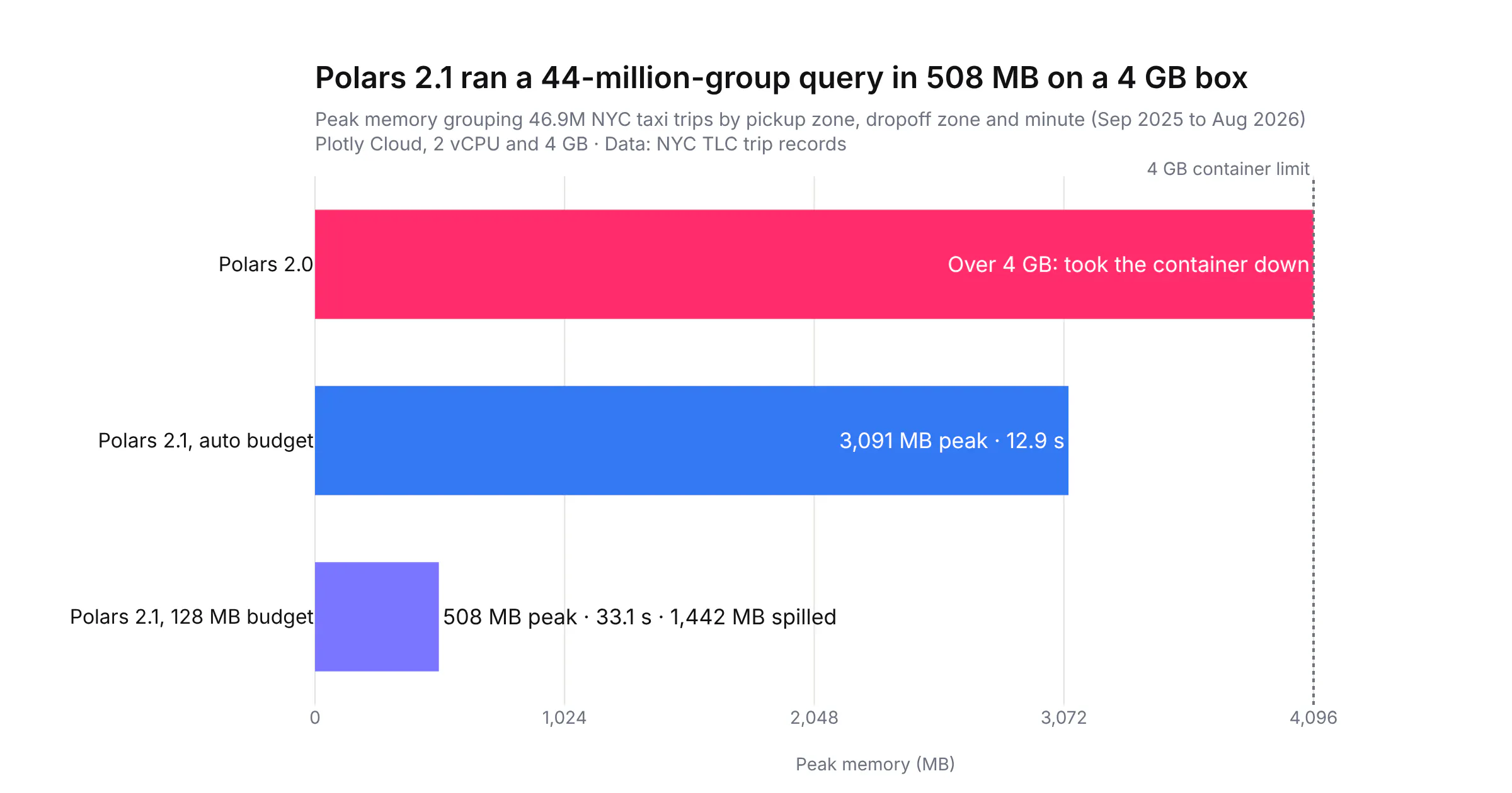
- This release closes the biggest gap left in that promise. Steps that have to remember the whole dataset, like a sort or a group-by with millions of distinct keys, still needed all of that state in memory. Polars 2.0 let sorts and window functions spill their state to disk, and 2.1 adds the group-by, which the Polars team calls the most common reason queries run out of memory. On a 4 GB Plotly Cloud box, Polars 2.1 grouped 46.9 million NYC taxi trips into 44.2 million groups at a 508 MB peak, while the same query on Polars 2.0 took the container down.
Here is how the Polars team's own changelog for 2.1 starts, as published in their release post on October 27, 2026. The issue numbers point at pull requests in the Polars repository.
Polars 2.1 is out. This post gives an overview of the highlights grouped by area. Everything else is in the release notes.Upgrade with:pip install -U polars## Before you upgradeTwo changes may need your attention:- #30071 – Disallow mixed string <=> numeric arithmetic in eager. pl.Series([1, 2]) + "4" used to return ["14", "24"] and now raises, as it already did in lazy- #29888 – Drop support for Python 3.10## Out-of-coreIn 2.0 we enabled spilling to disk by default, but the most common reason for running out of memory, a high-cardinality group-by, couldn't spill yet. Now it can.- #29911 – Run the streaming group-by out of core, with shuffles- #30282 – Evaluate the streaming window node (over) out of core- #30104 – Add an out-of-memory kill threshold (POLARS_OOMKILL_THRESHOLD_FRACTION)- #29259 – Add a reverse node to the streaming engine- #29792 – Add query-level IO active time and thread count metrics...
The full changelog goes on through SQL, Iceberg, Parquet, performance and bug fixes. The rest of this post picks out the parts we could test in Dash apps and runs them on real data.
Polars has always been about handling massive amounts of data on a single node. Instead of spreading a job across a cluster, it runs the whole query on one machine's cores and streams through the data. The Polars user guide sums up the idea: instead of processing all the data at once, Polars "can execute the query in batches allowing you to process datasets that do not fit in memory." A filter, a column selection or a sum over a few groups only needs the batch in front of it, so the size of the input stops mattering. For a Dash app, that means a callback can query far more data than the server it runs on could ever hold in memory.
Some steps have to remember things across the whole dataset, though. A sort has to see every row before it can return the first one, and a group-by keeps a running total for every distinct key it has seen. Streaming the input doesn't shrink that state, so a group-by over 44 million route-minutes runs out of memory on our 4 GB test box even though the input was never loaded all at once. The way around it is spilling, where the engine writes part of that state to disk and reads it back later. Without it, the fix on Polars was to buy a bigger box, or to hash-partition the keys by hand and aggregate one slice at a time.
Polars has been filling that gap in over the last two years. With Polars 1.0 in July 2024, the team said it was "completely redesigning our streaming engine", and the new engine was opt-in through 2025 while it caught up (tracking issue). Polars 2.0, released on October 6, 2026, made it the default for collect() and turned spilling on by default, starting at about 80% of RAM with a 64 GB disk budget. That first version covered "sort, window functions, many expressions", and the release post said joins and group-bys would follow. Polars 2.1 delivers the group-by, and the release post puts it plainly: "In 2.0 we enabled spilling to disk by default, but the most common reason for running out of memory, a high-cardinality group-by, couldn't spill yet. Now it can." The streaming node behind over() runs out of core in 2.1 as well. The 2.1 notes don't mention joins, so a join with a very large side can still run out of memory.
We built three Dash apps around the 2.1 release on real data (NYC yellow cab trips, OpenFlights routes and hourly weather), deployed them to one Plotly Cloud box with 4 GB of memory, and logged every timing. A box that size makes the memory limit easy to reach, so the difference between 2.0 and 2.1 shows up on a dataset we could download and rerun, and the same limits apply on a bigger machine with more data. For each feature we also checked that the new 2.1 code returns exactly what the 2.0 workaround returned.
We're big fans of Polars. Give 2.1 a try and let us know what you think:
pip install -U polars
How we tested Polars 2.1
All three apps run on Plotly Cloud's Standard 2x size (2 vCPU, 4 GB) and share one copy of the data on a persistent filesystem mounted at /data. On boot they download every NYC TLC yellow cab month from January 2023 to August 2026, which is 44 files and 157,904,393 trips (2.88 GB once normalized), plus the OpenFlights route graph and hourly Central Park weather from Open-Meteo.
We built three Dash apps, one for each part of the release we wanted to test. Spill Lab demonstrates and measures how spilling to disk works across a range of scenarios: it runs the same group-by or window query over anything from one month of trips to the full dataset, with different memory budgets, on Polars 2.0 or 2.1, and records the time, the peak memory and how much went to disk. SQL Atlas runs the new SQL features on flight routes and taxi trips, from recursive CTEs to ASOF JOIN. Parquet Vault writes and reads Parquet files with encrypted columns and times the faster scans.
Heavy queries run in their own subprocess. That way each app can read a query's peak memory, catch Polars' spill metrics from stderr, and survive an out-of-memory kill without losing the web worker. Each app runs a fixed benchmark on boot and logs every result, and for comparisons it loads Polars 2.0 from a side folder on the same box. Running queries in a separate process is our own choice for a benchmark app rather than something Polars or Dash asks for, and a section further down explains why we did it and what we'd recommend instead.
We used two more setups for things the Cloud apps don't cover. The app screenshots come from the same code running locally in a container capped at 4 GB and 2 CPUs, because the Cloud apps are private. The before-and-after checks (does the 2.1 code return the same answer as the 2.0 workaround?) ran in that same capped container on January to August 2025 taxi data, 31.6 million trips. Our scripts and logs are in the post's folder in our content repo.
Out-of-core group-by in Polars 2.1
A group-by keeps one running state per group, so its memory grows with the number of distinct keys rather than with the size of the data. Per-minute rollups, per-trade or per-account aggregates and readings per sensor per interval can produce almost one group per row. In 2.1, Polars' streaming group-by can spill that state to disk once it passes a memory budget.
Since spilling comes up a lot below, here it is in a bit more detail. When a query's working state grows past a memory limit, the engine writes part of it to temporary files on disk and reads it back when it needs it, so the query keeps going with far less memory instead of being killed. It's slower than keeping everything in memory, because disk is slower than RAM, but the query finishes. In Polars the limit is the memory budget, set with POLARS_OOC_MEMORY_BUDGET_MB (OOC stands for out of core, an older name for the same idea), and the temporary files go to the folder in POLARS_OOC_SPILL_DIR, which in our apps points at the persistent filesystem. "Spilled" in the tables below means how many megabytes went to disk that way.
Our stress test groups trips by pickup zone, dropoff zone and minute, which makes close to one group per trip:
lf = pl.scan_parquet("/data/polars21/tlc/clean/*.parquet")(lf.group_by(pl.col("pickup").dt.truncate("1m"), "pu", "do").agg(pl.len().alias("trips"),pl.col("fare").mean(),pl.col("do").n_unique().alias("destinations")).sink_parquet("/data/polars21/work/result.parquet"))
The budget is an environment variable, POLARS_OOC_MEMORY_BUDGET_MB, and POLARS_OOC_LOG_METRICS=1 prints how much was spilled. Here is that query over the 12 months from September 2025 to August 2026 (46.9 million trips, 44.2 million groups) on the 4 GB Plotly Cloud box:
Route by minute, 12 months
Wall time
Peak memory
Spilled
Polars 2.0
Container restarted
Over 4 GB
n/a
Polars 2.1, default budget
12.9 s
3,091 MB
9 MB
Polars 2.1, 128 MB budget
33.1 s
508 MB
1,442 MB
The default budget is the fastest choice when the groups fit, so it's the right setting for most queries. On all 44 months they didn't fit on this box. With the default budget, both full-dataset group-bys stopped at the out-of-memory threshold we set (more on that below), and Polars 2.0 took the container down.
A smaller budget is what gets the full dataset through. On the 4 GB Plotly Cloud box, with a 256 MB budget, Polars 2.1 grouped all 161.8 million trips (45 months by the time of this run, through September 2026) into 152.0 million groups. It peaked at 1,409 MB and spilled 5,178 MB to the persistent filesystem, and the app kept serving pages the whole time. The run took 12 minutes. In a local container capped at 4 GB and 2 CPUs, a 256 MB budget took 157.9 million trips into 148.4 million groups in 105 seconds, peaking at 1,319 MB and spilling 5,035 MB, which is the run in the screenshot below. We haven't profiled that gap yet. One difference is that the Cloud run wrote its spill files to the persistent filesystem, while the local run wrote them to the container's own disk.
Where the spill files go matters on Plotly Cloud and Dash Enterprise. Polars 2.1 writes them to the folder in POLARS_OOC_SPILL_DIR, and when that isn't set it uses /var/tmp, on the container's own disk. It ignores POLARS_TEMP_DIR, which is the variable we set at first. On Plotly Cloud, files on the container's own disk count against the app's memory, so our first full-dataset runs put about 5 GB of spill files into a 4 GB box and the container restarted 15 seconds in. Setting POLARS_OOC_SPILL_DIR to a folder on persistent storage fixed it:
os.environ["POLARS_OOC_SPILL_DIR"] = "/data/polars-spill"os.environ["POLARS_OOC_MEMORY_BUDGET_MB"] = "256"
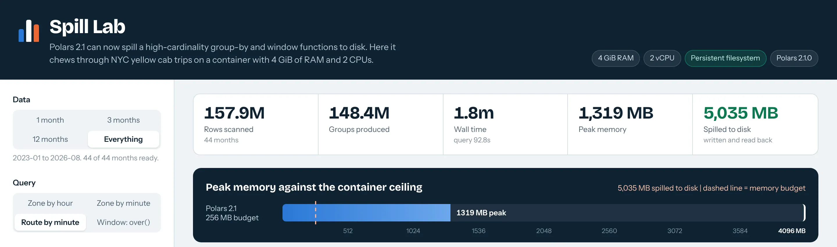
On smaller queries the budget costs very little. Three months grouped by zone and minute (10.7 million trips, 4.7 million groups) took 1.8 s at 931 MB with the default budget and 3.6 s at 324 MB with a 256 MB budget. Polars 2.0 needed 7.7 s and 1,268 MB for the same query on the same box.
Before 2.1: partition the keys yourself
Polars streamed the input, but when the groups themselves didn't fit in memory the query got killed, so the workaround was to hash-partition the keys and aggregate one slice at a time:
P = 8for p in range(P):(lf.filter(pl.col("k").hash(seed=0) % P == p).group_by("k").agg(pl.col("v").sum().alias("s"), pl.col("v").n_unique().alias("u")).sink_parquet(f"out/part_{p}.parquet"))
We compared it with the 2.1 version on the example from the Polars changelog: 30 million keys read from Parquet and written back to Parquet, in the 4 GB container. All four runs returned identical results:
30M-key group-by
Time
Peak memory
2.0, plain query
8.1 s
2,863 MB
2.0, hand-partitioned into 8 slices
9.6 s
590 MB
2.1, plain query
5.1 s
3,057 MB
2.1, same query, 200 MB budget
6.9 s
352 MB
The 2.1 version is the one-liner you'd write anyway, and with a budget it used less memory than our hand-rolled partitioning and finished faster, spilling 231 MB along the way.
Out-of-core window functions
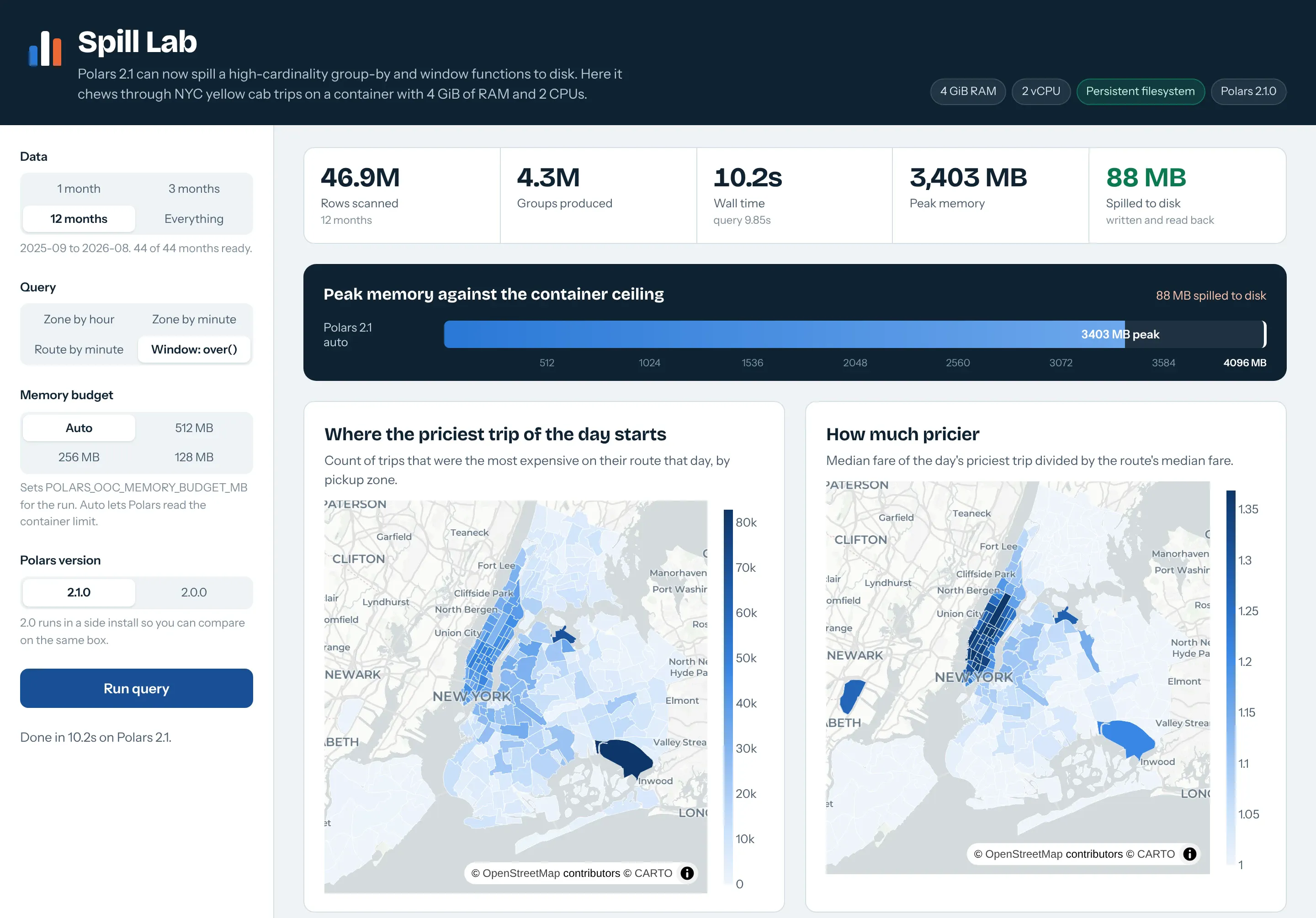
Window functions run into the same limit in a different shape. A function with over() computes something per partition, such as a rank within a route and day or a median per route, and with millions of partitions that state outgrows memory the same way a group-by does. In 2.1 the streaming window node behind over() can spill as well. Spill Lab's window mode ranks every fare within its route and day, keeps the day's most expensive trip on each route, and maps where those trips start:
day = pl.col("pickup").dt.date()(lf.filter(pl.col("fare") > 0).with_columns(pl.col("fare").rank("ordinal", descending=True).over("pu", "do", day).alias("rank_in_route_day"),(pl.col("fare") / pl.col("fare").median().over("pu", "do")).alias("vs_route_median")).filter(pl.col("rank_in_route_day") == 1).group_by("pu").agg(pl.len(), pl.col("vs_route_median").median()).sink_parquet("/data/polars21/work/result.parquet"))
On the Cloud box over 12 months (46.9 million trips, 4.3 million route-days), 2.1 with the default budget took 9.6 s, peaked at 3,532 MB and spilled 111 MB. Polars 2.0 ran the same query in 9.4 s at 3,453 MB. So at this size the window spilling didn't save memory on its own, and as with the group-by, a smaller budget is how you'd ask it to.
Stopping runaway queries with POLARS_OOMKILL_THRESHOLD_FRACTION
In a container with a hard memory limit, a query that grows past the limit gets killed by the operating system, and on Plotly Cloud or Dash Enterprise, where each app runs in its own container, that restarts the whole app rather than just the query. New in 2.1, POLARS_OOMKILL_THRESHOLD_FRACTION makes Polars stop a runaway query itself before that happens. Our job runner sets it to 0.85:
env = dict(os.environ,POLARS_OOC_LOG_METRICS="1",POLARS_OOMKILL_THRESHOLD_FRACTION="0.85")subprocess.run([sys.executable, "worker.py", task, params, result], env=env)
A query that crosses the line exits with polars: memory usage exceeded POLARS_OOMKILL_THRESHOLD_MB or POLARS_OOMKILL_THRESHOLD_FRACTION, aborting. That's what happened to the two all-months group-bys with the default budget on Plotly Cloud: each failed after 8 to 18 seconds with that message, and the app carried on serving pages. The Polars 2.0 runs of the same queries ignore the variable, and both times they took the whole container down until it restarted.
Before 2.1, you'd cap the process with resource.setrlimit (which breaks easily with allocators that reserve a lot of virtual memory) or run a watchdog thread that kills the job when its memory crosses a line. On a shared box, the difference between one failed query and a restarted app is a big one.
Recursive CTEs in Polars SQL
A recursive CTE is how SQL walks a graph or a hierarchy when you don't know in advance how many joins it will take. Think of a bill of materials down to the last part, a chain of corporate ownership, a pipeline network from a well to a terminal, or flight routes out of an airport. The query starts from a seed row and keeps joining its own result back onto a table until a stop condition is met. Recursive CTEs have been in the SQL standard since SQL:1999, and PostgreSQL, SQLite, MySQL 8, SQL Server and Oracle all support them. Polars SQL adds them in 2.1.
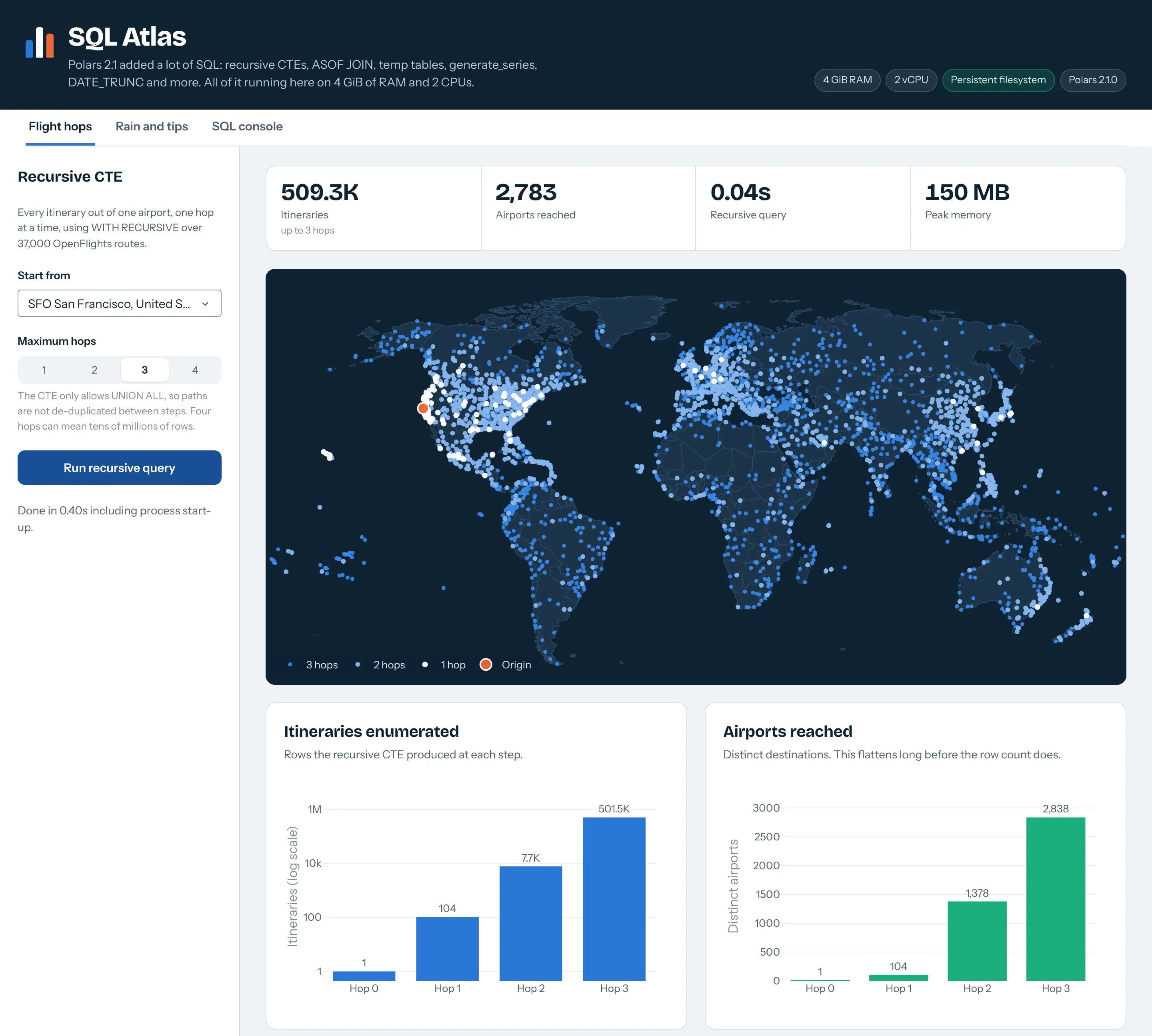
SQL Atlas uses WITH RECURSIVE to walk the 37,595 routes in OpenFlights and find every airport you can reach from one origin:
WITH RECURSIVE hops(iata, n) AS (SELECT 'SFO', 0UNION ALLSELECT r.dst, h.n + 1FROM hops h JOIN routes r ON r.src = h.iataWHERE h.n < 3)SELECT n, COUNT(*) AS itineraries, COUNT(DISTINCT iata) AS airportsFROM hops GROUP BY n
Before 2.1, Polars SQL had no recursion, so you'd drop to Python and expand the frontier with a loop of joins:
frontier = pl.DataFrame({"iata": ["SFO"]})steps = [frontier.with_columns(n=pl.lit(0))]for n in range(1, 4):frontier = (frontier.join(routes, left_on="iata", right_on="src").select(pl.col("dst").alias("iata")))steps.append(frontier.with_columns(n=pl.lit(n)))pl.concat(steps).group_by("n").agg(pl.len(), pl.col("iata").n_unique())
Both return the same counts for every hop. Three hops out of SFO produce 501,531 itineraries that reach 2,838 distinct airport codes. The CTE ran in 0.027 s and the loop in 0.042 s, so the gain here is keeping the whole thing in SQL rather than speed.
The CTE only accepts UNION ALL, so nothing gets deduplicated between steps and the row count multiplies with each hop. On Plotly Cloud, four hops out of SFO produced 33.6 million rows in 2.6 s at a 924 MB peak, and four hops out of JFK produced 56.0 million rows at 1,384 MB. Five hops out of SFO ran our 4 GB container out of memory.
Other engines also accept plain UNION, which drops duplicate rows at every step. On the same routes, SQLite 3.45 returns the same 509,293 rows as Polars for three hops with UNION ALL, and 4,321 rows with UNION. Until Polars accepts UNION, keep the hop count low, or deduplicate each step in a Python loop like the one above.
ASOF JOIN in Polars SQL
An as-of join matches each row to the most recent row in another table at or before its timestamp. An equality join can't do that, because timestamps from two sources rarely line up exactly. It's the standard way to attach the prevailing quote to each trade, the latest sensor reading to each event on a well, or the last lab result before each dose. kdb+ made it famous in trading with its aj function, pandas has merge_asof, and Snowflake and ClickHouse have ASOF JOIN in SQL. Polars has had it in the DataFrame API as join_asof, and 2.1 adds it to Polars SQL with the same MATCH_CONDITION syntax Snowflake uses.
SQL Atlas uses it to give every taxi trip the weather reading in effect when it started, after a temp table buckets the sky:
CREATE OR REPLACE TEMP TABLE wx ASSELECT ts, CASE WHEN precip_mm >= 2.5 THEN 'Heavy rain'WHEN precip_mm > 0 THEN 'Rain'ELSE 'Dry' END AS skyFROM weather;SELECT w.sky, COUNT(*) AS trips,AVG(CASE WHEN t.payment = 1 AND t.fare > 0 THEN t.tip / t.fare END) AS tip_rateFROM trips tASOF JOIN wx w MATCH_CONDITION (t.pickup >= w.ts)GROUP BY w.sky
Before 2.1, SQL couldn't do an as-of join, so this meant leaving SQL for the DataFrame API and sorting both sides yourself:
wx = weather.lazy().with_columns(sky_expr).sort("ts")(trips.sort("pickup").join_asof(wx, left_on="pickup", right_on="ts", strategy="backward").group_by("sky").agg(pl.len(), tip_rate_expr))
The SQL version sorts both sides for you. On Plotly Cloud, the join over 12 months of trips (46.9 million) took 4.7 s and peaked at 1,893 MB. For the before-and-after check we joined 31.6 million trips from January to August 2025 to NOAA's hourly Central Park record, since Open-Meteo had rate-limited us by then. Both versions put 29,044,671 trips in dry hours, 1,946,553 in rain and 565,053 in heavy rain, with tip rates identical to the ninth decimal, and they took 2.4 s and 2.5 s. Swapping pl.date_range for SQL generate_series also gave the identical 366-day calendar for 2024.
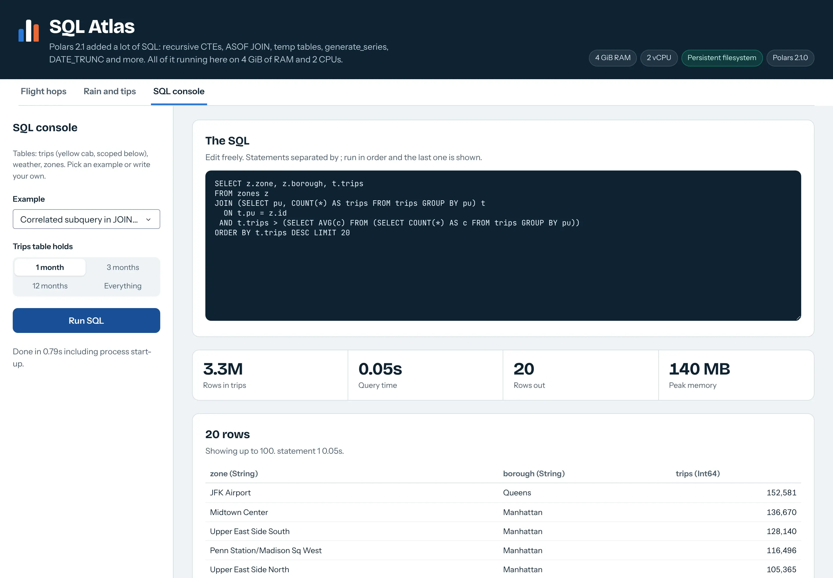
The release has more SQL than one app could hold: correlated and uncorrelated subqueries in JOIN ... ON, REGEXP_REPLACE, DATE_TRUNC, temp tables and more. SQL Atlas has a console tab with an example for each of those, and every one ran on 12 months of trips on Plotly Cloud in under 2.5 s.
Encrypted Parquet with a key per column
Parquet files travel. They get copied to object storage, shared with another team, attached to a ticket or kept in a backup, and whoever ends up with a file can read every column in it. Parquet's modular encryption, part of the Apache Parquet format, encrypts a file with AES and can use a separate key for each column, so one file can carry columns everyone may read next to columns only some people may. Spark (from 3.2) and PyArrow have supported it for a while. Polars 2.1 now reads and writes it, with a key per column if you want one.
Parquet Vault encrypts only the money columns and leaves the footer in plaintext, so anyone can read the schema and the other columns:
enc = pl.ParquetEncryptionProperties(footer_key=FOOTER_KEY,column_keys={"fare": FINANCE_KEY, "tip": FINANCE_KEY, "total": FINANCE_KEY},plaintext_footer=True,)lf.sink_parquet("/data/polars21/vault/trips_encrypted.parquet", encryption=enc)dec = pl.ParquetDecryptionProperties(footer_key=FOOTER_KEY,column_keys={"fare": FINANCE_KEY, "tip": FINANCE_KEY, "total": FINANCE_KEY},)pl.scan_parquet(path, decryption=dec).group_by("pu_borough").agg(pl.col("total").sum())
Before 2.1, Polars couldn't write encrypted Parquet, so you went through PyArrow's crypto factory, which wants a KMS client class even when you already hold the keys:
import pyarrow.parquet as pqimport pyarrow.parquet.encryption as peclass MyKms(pe.KmsClient):def wrap_key(self, key_bytes, master_key_id): ...def unwrap_key(self, wrapped_key, master_key_id): ...cf = pe.CryptoFactory(lambda cfg: MyKms(cfg))enc = cf.file_encryption_properties(pe.KmsConnectionConfig(), pe.EncryptionConfiguration(footer_key="footer", column_keys={"finance": ["fare", "tip", "total"]},plaintext_footer=True, double_wrapping=False))pq.write_table(df.to_arrow(), path, encryption_properties=enc)
Both routes round-tripped a million trips exactly, and both refused to read fare without a key. The Polars 2.1 version wrote and read back in 0.12 s, against 0.93 s through PyArrow. On Plotly Cloud, writing 12 months of trips (46.9 million) took 20.0 s encrypted and 20.3 s as plain Parquet, so the encryption itself cost nothing we could measure.
Reading as
Zone and trip columns
Fare, tip, total
Analyst, no keys
Readable
Refused: column is encrypted
Finance, right key
Readable
Readable
Wrong key
Refused
Refused
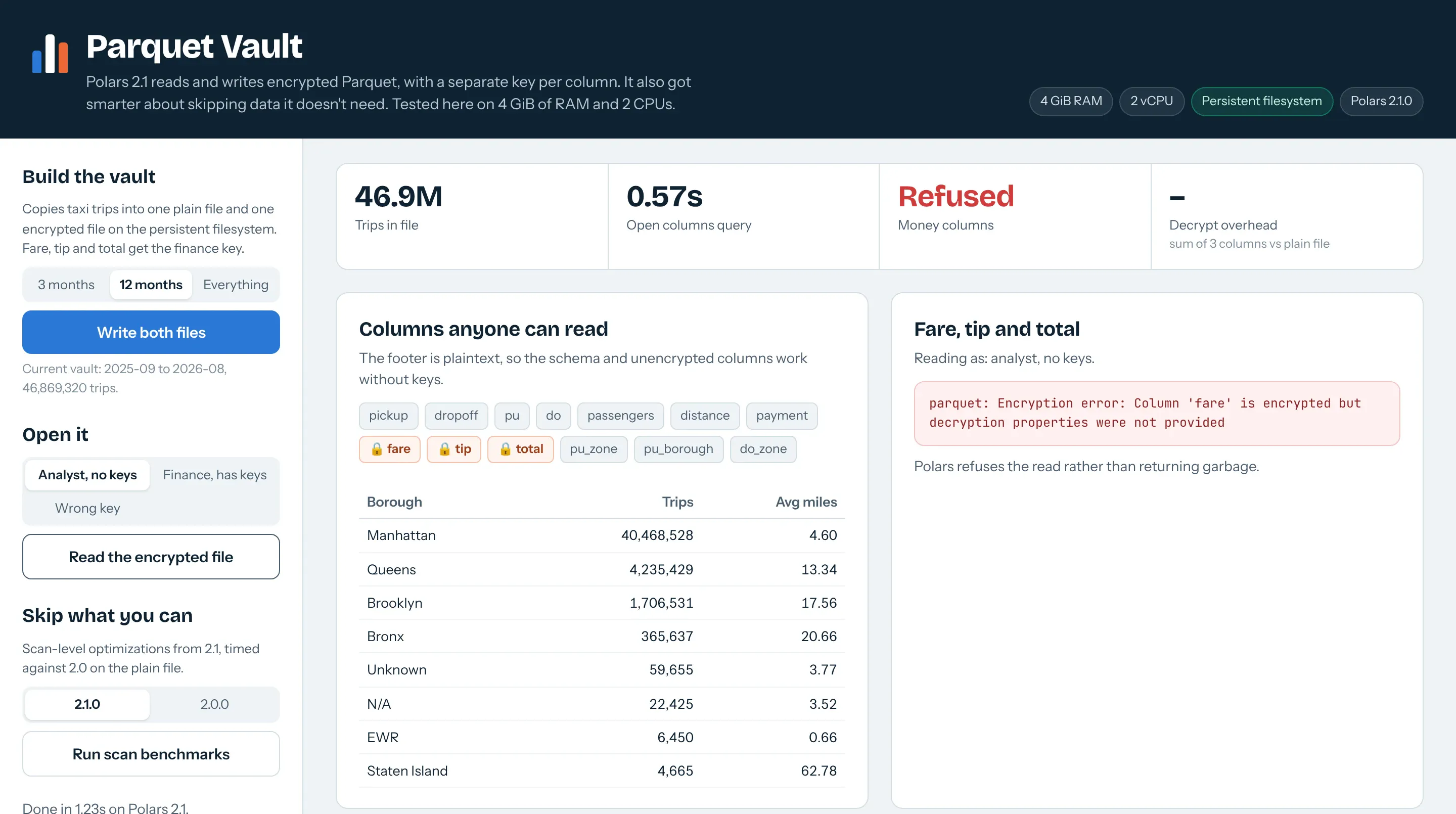
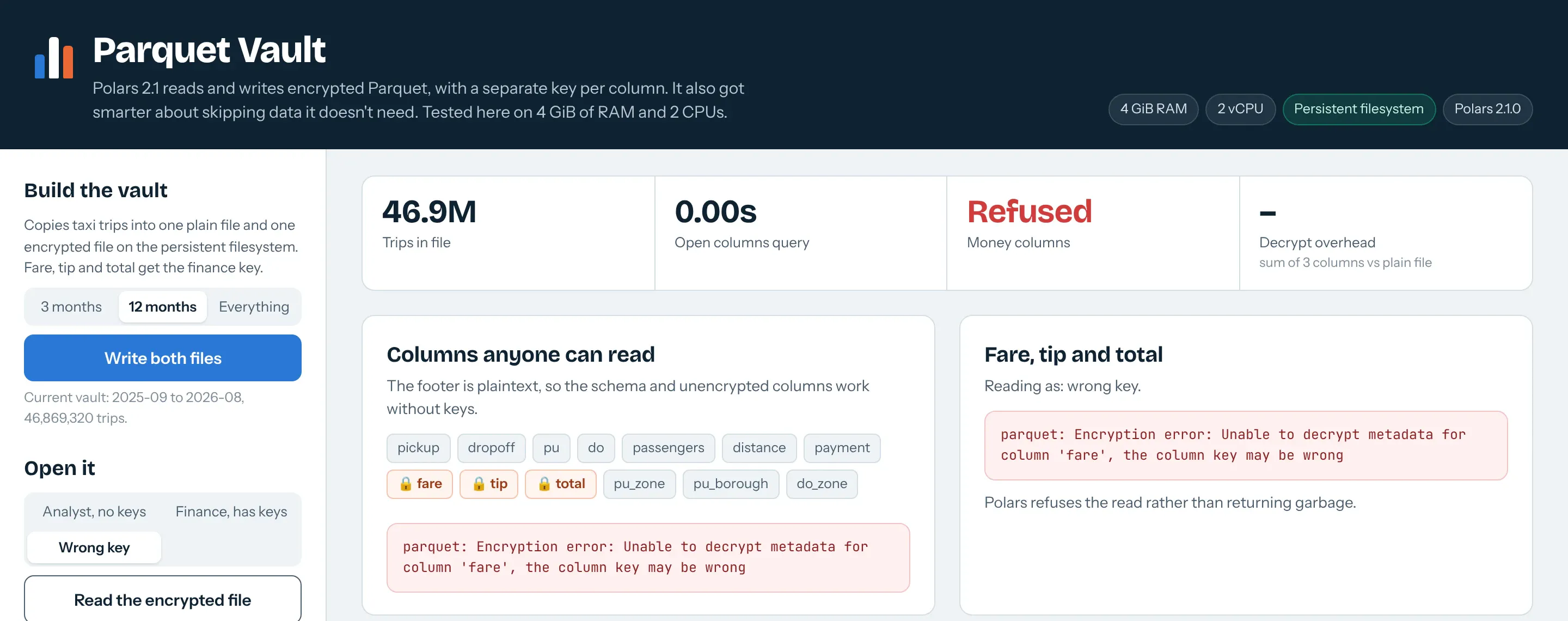
The wrong-key row surprised us. With no keys, the unencrypted columns read normally. With a wrong key for fare, even a query that only touches pu_borough fails with Unable to decrypt metadata for column 'fare'.
Setting up the keys on Plotly Cloud and Dash Enterprise
The keys are plain bytes, either 16 or 32 of them (Polars rejected 20 and 24), and in practice they live in environment variables. Generate one key for the footer and one for each group of columns you want to protect, and keep a copy in your password manager or secret store, because columns encrypted with a lost key can't be recovered:
python -c "import base64, secrets; print(base64.b64encode(secrets.token_bytes(32)).decode())"
In Plotly Cloud, open the app's Settings, go to the General tab, edit Environment variables, add PARQUET_FOOTER_KEY and PARQUET_FINANCE_KEY, and select Save and restart, which creates a new revision with the variables applied. On Dash Enterprise, add the same two variables to the app's environment variables in its settings. The app then reads them like any other setting:
import base64, osFOOTER_KEY = base64.b64decode(os.environ["PARQUET_FOOTER_KEY"])FINANCE_KEY = base64.b64decode(os.environ["PARQUET_FINANCE_KEY"])
Give the finance key only to the apps that should see the money columns. An app that never has PARQUET_FINANCE_KEY in its environment can't decrypt them, whatever its code does. Our demo keeps every key in one app and switches roles in the UI, which shows the behavior, but in a real setup the separation comes from which app holds which key.
Why not encrypt the whole file?
You could encrypt the whole Parquet file yourself, with GPG or an encrypted zip, or lean on encryption at the storage level, like encrypted disks or server-side encryption in S3. Both have gaps that per-column keys close.
If the whole file is encrypted with one key, anyone who needs any column needs that key, and then they can read every column. To keep the money columns from the analysts, you'd write a second copy without them and keep the two copies in sync. With a key per column, one file serves the analysts and the finance team, as the first two rows of the table above show.
A file encrypted as a whole also stops being Parquet until someone decrypts it. Every reader has to decrypt the full file to disk or memory first, so Polars can't scan it in place or read only the columns a query asks for. Parquet's own encryption works on each column separately inside the file, so Polars still opens it with scan_parquet and reads only what the query needs, which is how the analyst query above reads the zone columns of a file whose money columns it can't decrypt.
Storage-level encryption protects the disk, not the file. Anyone with read access to the bucket or folder gets the data decrypted, and once the file is copied somewhere else it's plain again. Parquet encryption travels with the file wherever it's copied.
If even the column names and row counts are sensitive, set plaintext_footer=False and the footer is encrypted too. Then nobody can read the file without the footer key, which is close to encrypting the whole file, while the money columns can still need a second key.
What it protects you from
It protects the file itself. Someone who gets a copy of the Parquet file, from the persistent filesystem, a bucket, a backup or an email, can't read the encrypted columns without the key. With a plaintext footer they still see the schema and the open columns. That's what lets one file serve two groups of people: analysts without the finance key read the zone and trip columns, and the finance team, who hold the key, also read fare, tip and total. The Parquet format's default algorithm, AES-GCM, also detects tampering with the encrypted parts.
It doesn't protect data once an app has decrypted it. Anyone who can open an app that holds the key sees what that app shows, so the app's sharing settings on Plotly Cloud or Dash Enterprise still decide who sees the money, and so do the settings for who can edit the app, since that's where the keys live. A plaintext footer also still shows the column names and row counts. Changing a key means rewriting the files that use it.
Faster Parquet scans
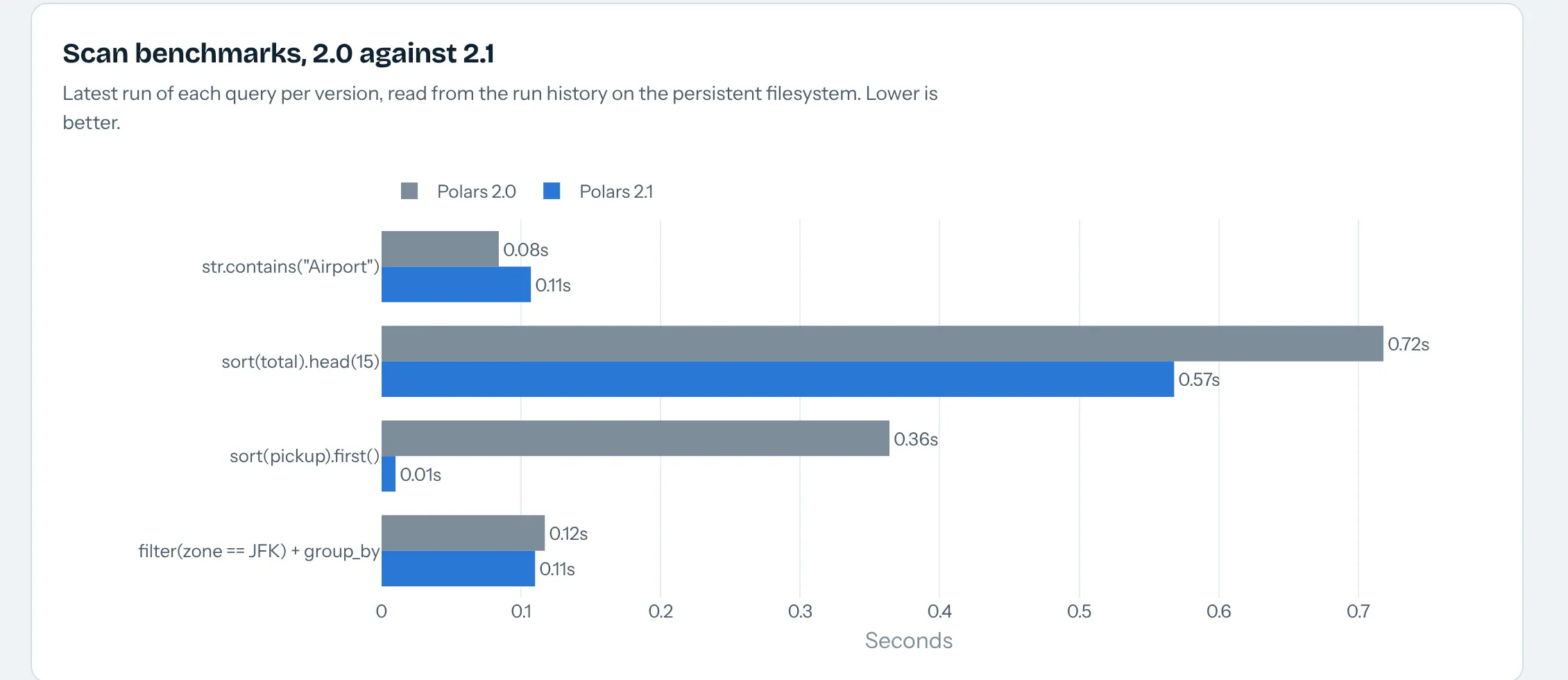
A lot of a release's performance work goes into reading less of each file: skipping row groups that can't match a filter, and rewriting a query into a cheaper one that gives the same answer. We timed four everyday queries on 2.1 and 2.0 against the same 12-month Parquet file (46.9 million trips) on Plotly Cloud, each on its second run:
lf.filter(pl.col("pu_zone").str.contains("Airport", literal=True)).select(pl.len())lf.sort("total", descending=True).head(15)lf.sort("pickup").select(pl.col("pickup").first())lf.filter(pl.col("pu_zone") == "JFK Airport").group_by("do_zone").agg(pl.len())
Query
Polars 2.0
Polars 2.1
str.contains("Airport", literal=True)
0.067 s
0.067 s
sort("total").head(15)
0.638 s
0.512 s
sort("pickup").first()
0.309 s
0.015 s
Equality filter and group-by
0.095 s
0.093 s
The big one is sort().first(), which 2.1 rewrites into a min() and runs about 20 times faster. Top-k got about 20% faster. The string prefilter and the plain filter didn't move on this file. In our 4 GB local container on a different 8 months of data, the sort().first() rewrite gave the same kind of jump (0.016 s against 0.247 s), while the other three came out about even with 2.0.
GeoParquet
GeoParquet is the standard way to store points, lines and polygons in Parquet. The geometry goes in a binary column, and a geo entry in the file's metadata records the encoding and the coordinate reference system, so tools like GeoPandas and GDAL know what they're reading. It's a common format for things like well locations, pipeline routes and lease blocks. Support in Polars 2.1 is experimental and lives behind two environment variables, with no Python API yet. POLARS_GEOPARQUET_READ=1 parses the geo footer, and POLARS_GEOPARQUET_WRITE=1.1 (or 1.0) writes one, attaching GeoArrow metadata to the geometry columns.
We tried it on the 6,072 OpenFlights airports that have an IATA code, written as GeoParquet by GeoPandas: read them with Polars, keep the 1,251 in the United States, write them back, and open the result in GeoPandas.
# POLARS_GEOPARQUET_WRITE=1.1 set in the environment(pl.scan_parquet("airports.parquet").filter(pl.col("country") == "United States").sink_parquet("us_airports.parquet"))gpd.read_parquet("us_airports.parquet") # 1,251 points, WGS 84
Writer
geo footer written
GeoPandas reads it
Polars 2.0
No
No: missing geo metadata
Polars 2.1, no flag
No
No: missing geo metadata
Polars 2.1, POLARS_GEOPARQUET_WRITE=1.1
Yes, version 1.1.0, WKB, CRS kept
Yes, 1,251 points
Before 2.1, a Polars filter in the middle of a geo pipeline stripped the geo footer, so you'd round-trip through GeoPandas or PyArrow just to put it back. Polars 2.0 already read GeoPandas' geometry column as a geoarrow.wkb extension type with the CRS, because GeoPandas embeds the Arrow schema. The new part is the write side, which makes Polars a safe middle step between GeoPandas and a Dash map. The geometry_types list comes back empty in the footer it writes.
The environment variables come from Polars PR #29987, "Add experimental geoparquet read/write", and the PR describes them as mainly there for the GeoPolars plugin rather than for everyday use. It only attaches GeoArrow metadata to the right columns, drops bounding boxes and orientation for now, and doesn't support GeoParquet 0.x or 2.x. GeoPolars, the Polars project's geospatial extension, is where the user-facing API is meant to land. Its README says it was long blocked on Polars supporting Arrow extension types, which Polars has since added, and that it is still a prototype that isn't production-ready. The maintainers are working on a rewrite with native GeoArrow types, CRS-aware operations and GeoParquet reading and writing, and want the API to settle before publishing it to PyPI (issue #279). GeoParquet in GeoPolars is tracked in issue #266, and GeoParquet 2.0 in issue #276. If you need spatial operations in Polars today, the community plugin polars-st builds on GEOS and stores geometries as binary columns.
Other changes worth knowing
We didn't test the Iceberg changes. sink_iceberg has a new partition_overwrite option, and there's a new Expr.truncdiv for integer division that rounds toward zero (-7 truncdiv 2 is -3, where // gives -4). Before you upgrade, note that Polars 2.1 needs Python 3.11 or newer, where 2.0 still installed on Python 3.10.
Why we ran Polars in a separate process
Every heavy query in these apps runs in its own Python process instead of inside the Dash callback. That's our own setup for a benchmark app, not something Polars or Dash requires, and most apps shouldn't copy it.
We did it for three reasons. A fresh process gives a clean peak-memory number for each query, which a long-lived web worker can't. One Python process can only import one version of Polars, and we wanted 2.0 and 2.1 side by side in the same app. And when a query runs out of memory, the operating system kills the worker process instead of the web worker that serves pages. Settings like the memory budget are environment variables, so a fresh process per run also lets each run use its own budget.
Here's the core of it, slightly simplified from the app code:
def start_job(task, params, budget_mb=None):job_id = uuid.uuid4().hex[:10]pfile, rfile = SCRATCH / f"{job_id}.params.json", SCRATCH / f"{job_id}.result.json"pfile.write_text(json.dumps(params))env = dict(os.environ, POLARS_OOC_LOG_METRICS="1", POLARS_OOMKILL_THRESHOLD_FRACTION="0.85")if budget_mb:env["POLARS_OOC_MEMORY_BUDGET_MB"] = str(budget_mb)def run():proc = subprocess.run([sys.executable, "worker.py", task, str(pfile), str(rfile)],env=env, capture_output=True, text=True)... # read rfile, parse spill stats from proc.stderr, write a status filethreading.Thread(target=run, daemon=True).start()return job_id # a dcc.Interval polls the status file until the job is done
Passing data in and out. Parameters go to the worker as a JSON file, and Polars settings as environment variables. The worker writes a small JSON result (counts, timings and the rows a chart needs) and writes anything large to Parquet on the persistent filesystem. Nothing the user types is pasted into a command line.
Security. The command is a list of arguments with no shell, so user input can't turn into shell commands. A separate process isn't a sandbox, though. The worker runs as the same user, sees the same files and has the same environment variables, encryption keys included. That matters most for SQL Atlas's console, which runs whatever SQL you type, because Polars SQL can read any file the process can reach with read_parquet('...'). That's acceptable in a private app for our own team. In a shared app you'd restrict the console, or run the worker somewhere that only has the data it needs.
Downsides. Every run starts Python and imports Polars before doing any work, and end to end that added 0.2 to 0.6 s per query on the Cloud box (a generate_series query took 0.005 s to run and 0.21 s in total). Nothing stays in memory between runs, so each query rescans its Parquet files, and results have to be written to files and read back. The job status files live in the container's /tmp, so this doesn't work across several containers unless you move them to something shared, like Redis.
Scale. Each app runs one heavy job at a time and turns away a second one with a message, because two at once would compete for the same 4 GB and two CPUs. Each worker process also starts its own Polars thread pool, so if you run several at once, cap them with POLARS_MAX_THREADS.
What we'd recommend instead. For most Dash apps, call Polars directly in the callback. Polars runs queries on its own thread pool, so a query that takes a second or two is fine there. For longer ones, Dash has background callbacks, which do the same job with less code. The DiskCache backend runs the callback in a separate process, and for production the Dash docs recommend the Celery backend with Redis, which queues jobs and runs them on dedicated workers. Our runner is close to the DiskCache approach, with extra plumbing for the measurements this post needed.
Things we tripped over
None of these took more than a few minutes to work around, and most are the kind of thing you only find on day one.
- The changelog's own spill example raises. Two aggregations on v with no alias give DuplicateError: column with name 'v' has more than one occurrence. Add .alias("s") and .alias("u") and it runs.
- Spill files ignore POLARS_TEMP_DIR. Polars 2.1 writes them to POLARS_OOC_SPILL_DIR, or to /var/tmp on the container's own disk if that isn't set. Our first full-dataset runs on Plotly Cloud spilled about 5 GB there, which counts against memory, and the container restarted. Pointing POLARS_OOC_SPILL_DIR at the persistent filesystem fixed it.
- Recursive CTEs only take UNION ALL. Plain UNION is refused with recursive CTE only supports UNION ALL, so there's no dedupe between iterations and paths multiply fast.
- EXTRACT(EPOCH FROM interval) isn't supported yet. Subtracting two EXTRACT(EPOCH FROM ts) calls works.
- A wrong column key breaks the whole read, as described above, even for columns that aren't encrypted.
- GeoParquet has no Python API yet. It's switched on with the POLARS_GEOPARQUET_READ and POLARS_GEOPARQUET_WRITE environment variables, and the user-facing API is meant to come through GeoPolars (see the GeoParquet section for where to follow it).
- On Plotly Cloud's 1 GB Starter size, the container's own disk counts against memory. Our first deploy wrote taxi months to local disk and got restarted every 110 seconds, right after the 7th month (about 900 MB). Moving data, spill files and query results to the persistent filesystem fixed it. If you're going to spill, spill to /data.
- Plotly Cloud's auto-sleep is request-based, so a long benchmark in a background thread needs the app kept awake. Our apps can't reach their own public URL from inside Plotly Cloud, so a self-ping didn't work.
How to build these apps yourself
Each app came out of a short prompt to a coding agent connected to Plotly Cloud. Start with the shared foundation, then paste the prompt for the app you want. The prompts below describe exactly what we deployed, and the same apps run on Dash Enterprise.
Shared foundation
Build a small shared Python module for Dash apps on Plotly Cloud. Use /data if it's mounted and writable, otherwise ./data. Download NYC TLC yellow taxi Parquet files from Jan 2023 to two months ago, normalize each month into a sorted Parquet file with zone names joined in, and delete the raw file afterwards. Run that download in a background subprocess with a file lock that has a heartbeat, so a container that dies doesn't hold the lock forever. Add a job runner that runs heavy Polars work in a subprocess, sets POLARS_OOC_LOG_METRICS=1 and POLARS_OOMKILL_THRESHOLD_FRACTION=0.85, points POLARS_OOC_SPILL_DIR at /data, parses spill stats from stderr, records peak memory, and appends every run to an NDJSON file on /data. Log every timing as a single "[p21] event=... key=value" line.
Spill Lab: out-of-core group-by and window functions, with a memory gauge and a 2.0 comparison.
Using that module, build a Dash app that runs a Polars streaming group-by over the taxi data. Let me choose the data range (1, 3 or 12 months, or everything), the group key (zone by hour, zone by minute, or zone pair by minute), a memory budget (auto, 512, 256 or 128 MB) and the Polars version (2.1 or 2.0, with 2.0 unpacked from PyPI wheels into a side folder). Show rows scanned, groups, wall time, peak memory and MB spilled. Make the hero a dark memory gauge that draws each run's peak against the container's memory ceiling. Add a window mode that ranks every fare within its route and day using over() and maps the result by taxi zone. Keep the run history on /data and plot it.
SQL Atlas: recursive CTEs, ASOF JOIN, temp tables, generate_series and a SQL console.
Build a Dash app with three tabs, all in Polars SQL. Tab one: a WITH RECURSIVE CTE over OpenFlights routes that finds every airport reachable from a chosen origin in up to N hops, drawn on a dark world map colored by hop count. Tab two: ASOF JOIN ... MATCH_CONDITION between taxi trips and hourly Open-Meteo weather for Central Park, bucketed with a CREATE TEMP TABLE, showing trips per hour, tip rate and speed by sky condition, plus a daily series built on generate_series. Tab three: a SQL console with examples for REGEXP_REPLACE, DATE_TRUNC, correlated subqueries in JOIN ON and temp tables. Show the exact SQL next to each result.
Parquet Vault: column-level Parquet encryption and scan benchmarks against 2.0.
Build a Dash app that writes the taxi data twice to /data: once as plain Parquet and once with pl.ParquetEncryptionProperties, encrypting only fare, tip and total with a column key and leaving the footer in plaintext. Let me read the encrypted file as an analyst with no keys, as finance with the right key, or with a wrong key, and show what each can see. Add a benchmark that times literal str.contains, sort().head() top-k, sort().first() and an equality filter on the plain file, on Polars 2.1 and 2.0, and charts them side by side.
Our Polars 2.0 post covers the previous release the same way.
Summary
Polars 2.1 lets a single machine finish group-bys whose state doesn't fit in its memory. With a memory budget, a 4 GB Plotly Cloud app grouped 46.9 million trips into 44.2 million groups at a 508 MB peak, where Polars 2.0 took the container down. The SQL additions let you keep recursive queries and as-of joins in SQL, with the same answers as the old DataFrame workarounds, and per-column Parquet encryption no longer needs PyArrow. Set the budget yourself when your data can outgrow the box, and keep POLARS_OOMKILL_THRESHOLD_FRACTION on so a runaway query fails on its own instead of taking the app with it. Thanks to the Polars team for another great release.