Chris Parmer

November 12, 2026

Piper Diagrams - A Complete Guide

TL;DR

A Piper diagram shows the major dissolved ions in a water sample on three linked panels: a triangle for the cations (calcium, magnesium, sodium plus potassium), a triangle for the anions (chloride, sulfate, bicarbonate plus carbonate) and a diamond above them that combines both, so each sample becomes three dots and its position in the diamond tells you what kind of water it is.
Piper diagrams are also known as trilinear diagrams and Hill-Piper diagrams, and are similar to ternary plots, Stiff diagrams and Durov diagrams, which are compared below.
Piper diagrams plot each ion as a percent of the total charge, measured in milliequivalents per liter (meq/L), so they show the kind of water and not how much dissolved salt it holds. This guide explains the unit and shows how to add the amount back.
You can make a Piper diagram with Plotly from scatter points on one pair of equal-scale axes, with the triangle and diamond outlines drawn as lines. The Python and plotly.js code below does that in about 30 lines.

What is a Piper diagram?

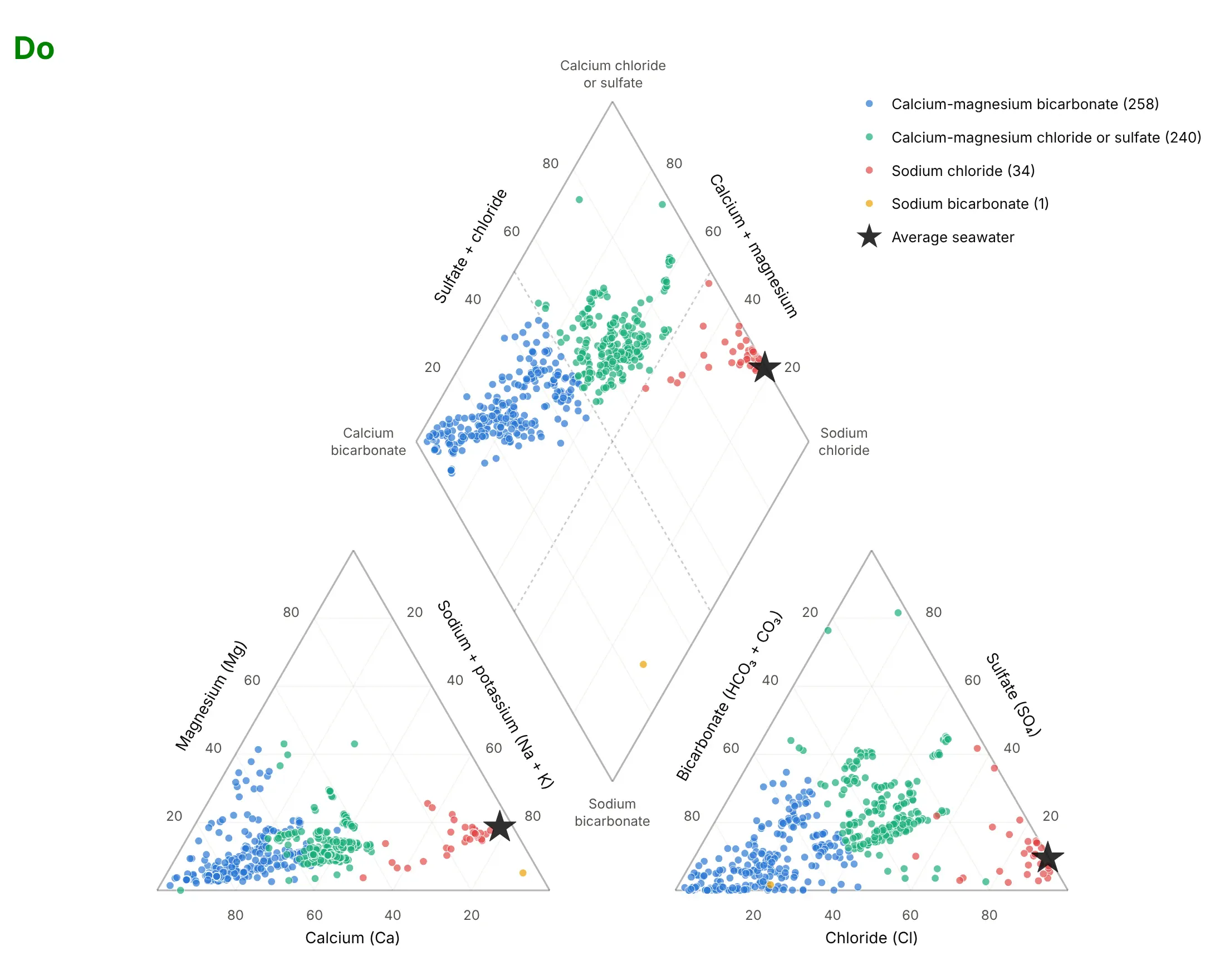
Piper diagrams look like this:

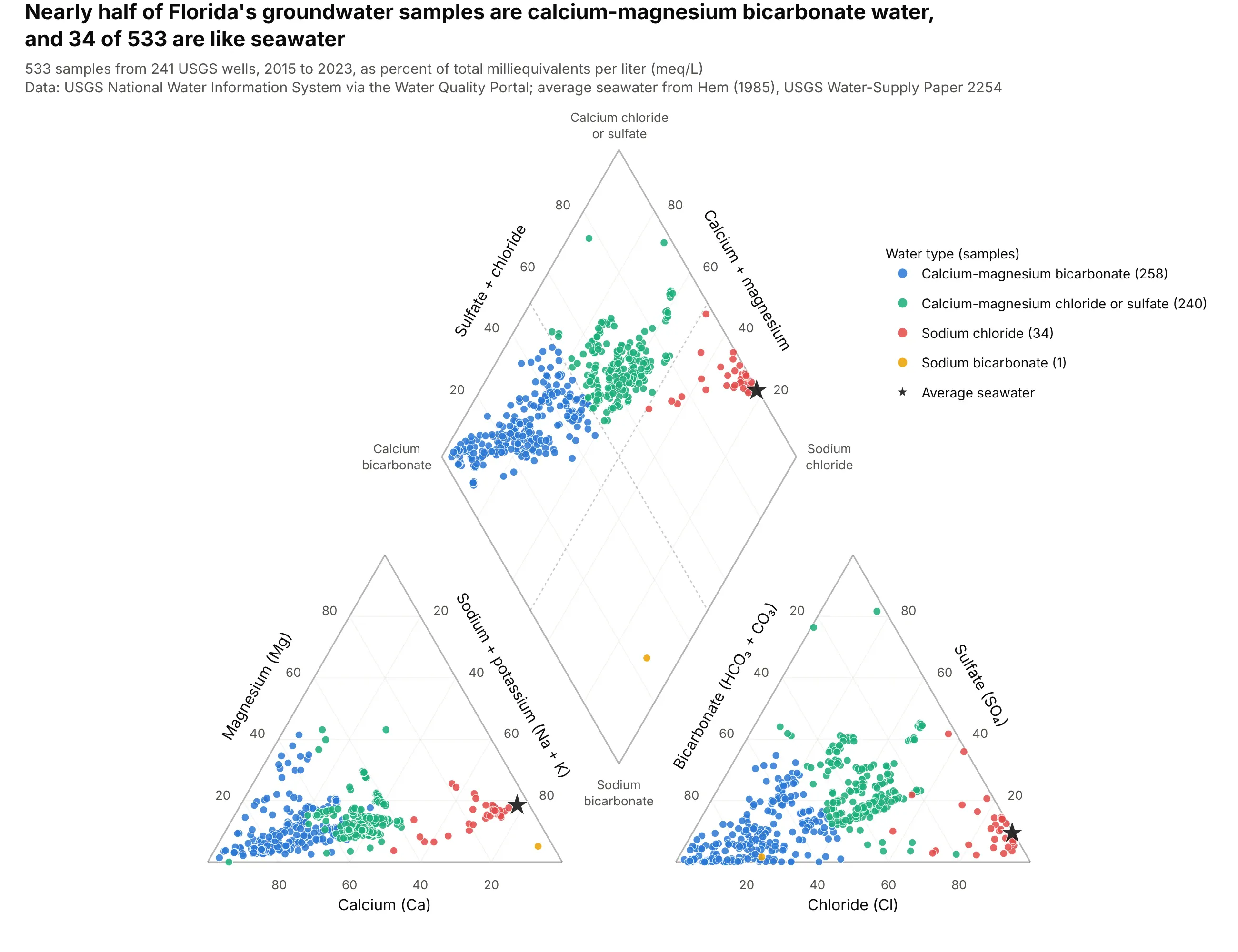
Piper diagram of 533 groundwater samples from 241 Florida wells: 258 calcium-magnesium bicarbonate samples in blue near the left corner of the diamond, 240 calcium-magnesium chloride or sulfate in green in the middle, and 34 sodium chloride samples in red beside a black star for average seawater at the right

Data: U.S. Geological Survey (USGS) National Water Information System (NWIS) via the Water Quality Portal; average seawater from Hem (1985), USGS Water-Supply Paper 2254.

How do you read a Piper diagram? In the example above, notice these things:

Each sample is drawn three times, once in the cation triangle at lower left, once in the anion triangle at lower right and once in the diamond, and the three dots have the same color. The diamond is the summary, and the triangles show which ions put the dot there.
The corners of the diamond name the water types. A dot near the left corner is calcium bicarbonate water, typical of limestone aquifers, and a dot near the right corner is sodium chloride water, like seawater. Florida's 258 calcium-magnesium bicarbonate samples (blue) have a median of 71% calcium among the cations and 73% bicarbonate among the anions.
The black star is average seawater at 78% sodium plus potassium and 90% chloride. The 34 red samples (median 71% sodium plus potassium and 85% chloride) sit next to it in all three panels, which is how a Piper diagram flags salty wells.
The dotted lines in the diamond are the 50% lines that split it into four water types. The 240 green samples have more than half of their cations as calcium plus magnesium but a median of 62% chloride plus sulfate among the anions, so they fall in the upper quadrant. Only 1 sample is sodium bicarbonate, and the lower half of the diamond is almost empty.
Every point is a percent of its own panel's total, so a sample with 10 times the dissolved salt lands in the same place as a dilute one with the same proportions. That is the main limit of the chart, and the produced-water and saline-lake examples show ways to add the amount back.

It's often used for charts like these:

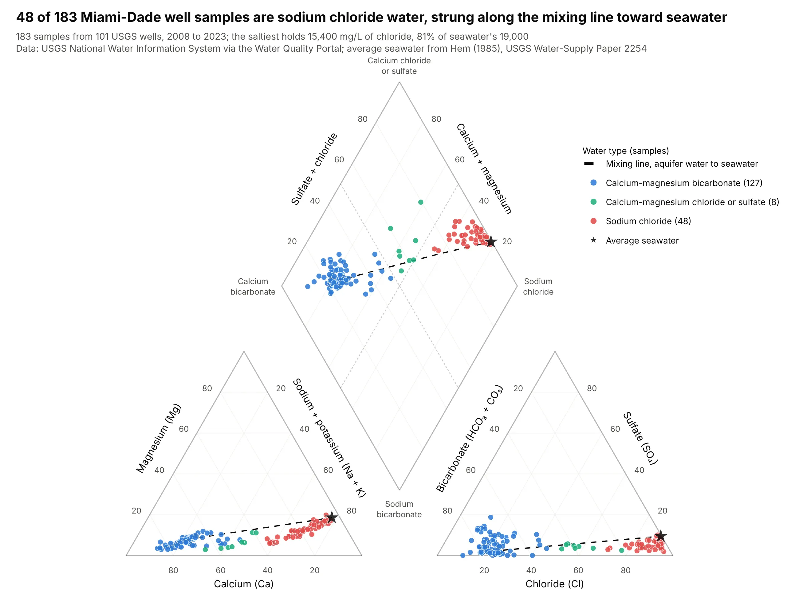
Piper diagram of 183 Miami-Dade County well samples: 127 calcium-magnesium bicarbonate samples clustered at the left corner, 8 in the middle and 48 sodium chloride samples at the right, all on a dashed mixing line that ends at a black star for average seawater

Seawater intrusion. 48 of 183 Miami-Dade well samples are sodium chloride water, and the saltiest holds 15,400 milligrams per liter (mg/L) of chloride, 81% of seawater's 19,000. Mixing two waters moves a sample along a straight line between them in every panel, so wells that are being invaded by seawater line up between the freshwater cluster and the star. The chart keeps 183 of 1,709 sample rows: 1,524 rows lack a complete set of major ions (most report chloride alone), and only 2 of the 185 complete analyses fail the 10% charge balance check. Data: USGS NWIS via the Water Quality Portal; seawater from Hem (1985).

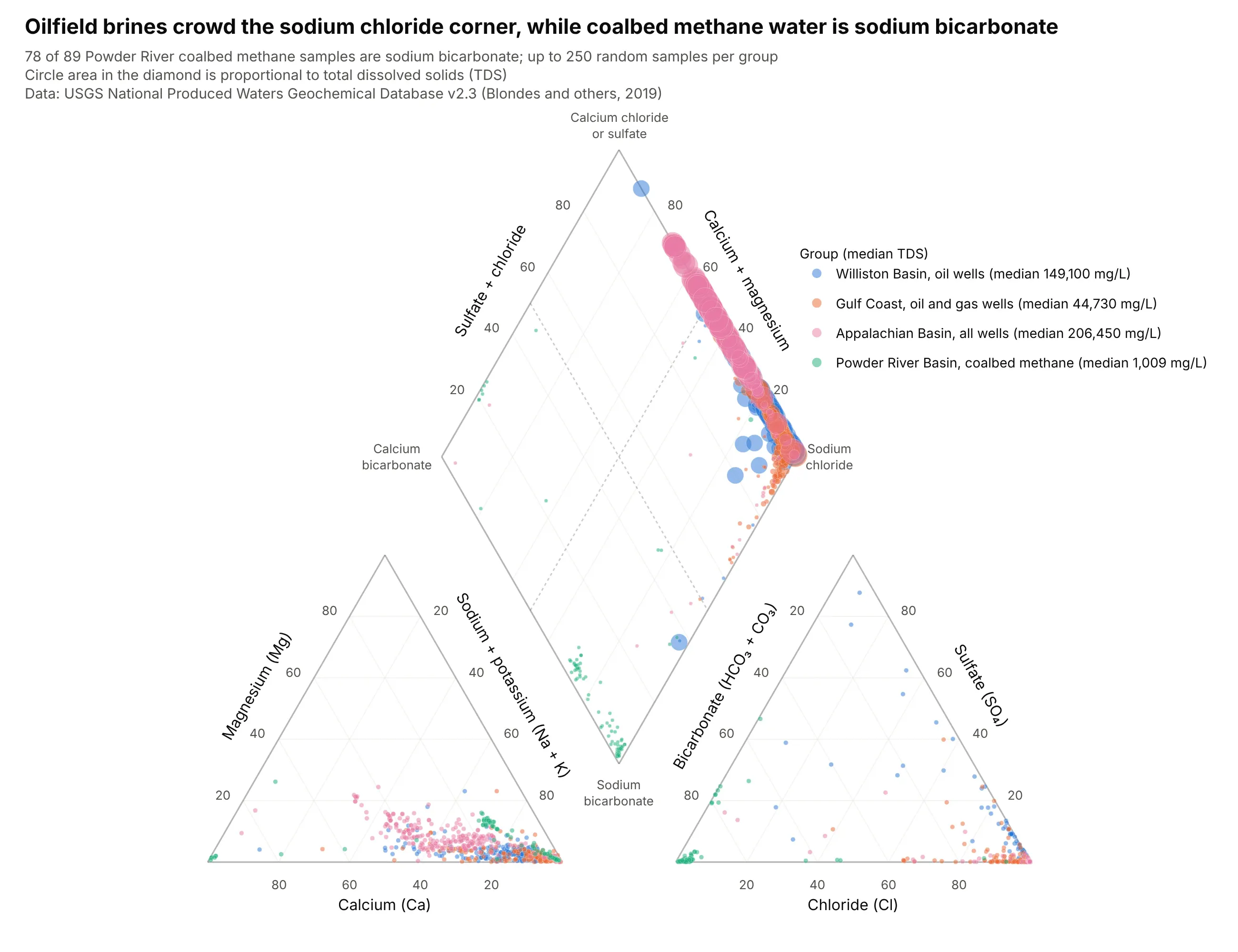
Piper diagram of produced water from four groups of wells: oilfield brines from the Williston, Gulf Coast and Appalachian basins crowd the sodium chloride corner with large circles in the diamond, while 78 of 89 Powder River coalbed methane samples sit at the sodium bicarbonate corner as small dots

Oil, gas and coal wells. Williston Basin oilfield brine has a median of 149,100 mg/L of total dissolved solids (TDS), against 1,009 mg/L for coalbed methane water in the Powder River Basin, and the two sit at opposite corners. Piper's own device of circles whose area follows TDS, used in the diamond here, adds the amount that percentages leave out. Data: USGS National Produced Waters Geochemical Database v2.3.

A short history

The Piper diagram builds on an earlier trilinear plot by R. A. Hill (Hill, 1940), which is why it is also called the Hill-Piper diagram. Arthur M. Piper added the diamond, which lets one point stand for the full analysis, and described the method in 1944 in the Transactions of the American Geophysical Union (Piper, 1944). The Groundwater Project's karst aquifer book notes that trilinear plotting systems have been in use since the early 1900s. The original 1944 data are not reproduced here, so this guide draws the method with current USGS data, and takes its average seawater from the USGS handbook Hem (1985).

Milliequivalents and percent, explained

Water analyses are reported in milligrams per liter (mg/L), the mass of each dissolved ion in a liter of water. A Piper diagram uses milliequivalents per liter (meq/L), which count electrical charge instead of mass. One equivalent is the mass of an ion that carries one mole of charge, so it is the ion's atomic or formula weight divided by its charge: sodium (22.99 g per mole, charge +1) is 22.99 g per equivalent, while calcium (40.08 g per mole, charge +2) is 20.04 g per equivalent. Dividing mg/L by that number gives meq/L.

Charge is the right currency because water is electrically neutral. The cations in a sample, added up in meq/L, must equal its anions, and a gap larger than about 10% of the total usually means a missing ion or an analysis error, which is why the examples here drop samples above that charge balance error. Mass hides this balance: average seawater holds 3.3 times more magnesium than calcium by mass but 5.4 times more by charge, because magnesium is the lighter ion.

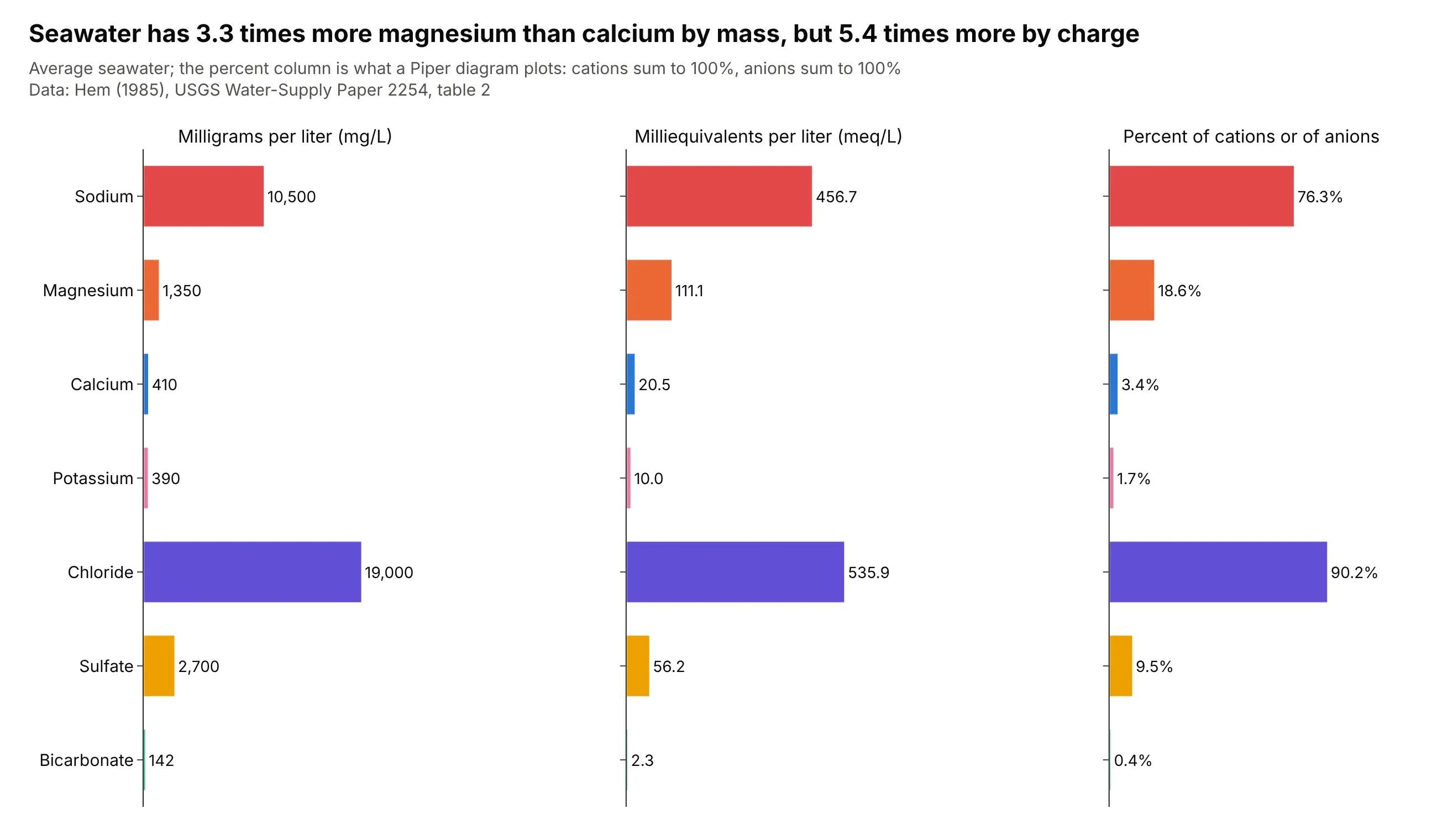
Three bar charts of average seawater: milligrams per liter, milliequivalents per liter and percent, with sodium at 10,500 mg/L, 456.7 meq/L and 76.3 percent of cations, and chloride at 19,000 mg/L, 535.9 meq/L and 90.2 percent of anions

The last step is percent. Each cation is divided by the total cations and each anion by the total anions, so each triangle's three values add to 100%. Those percentages are the coordinates: sodium plus potassium is 78.0% of the cations in seawater, chloride is 90.2% of the anions, and the diamond position follows from the sodium plus potassium share and the chloride plus sulfate share. Bicarbonate is usually estimated from alkalinity, which USGS reports as milligrams per liter of calcium carbonate, so the conversion there divides by 50.04 per equivalent.

Hydrochemical facies

The diamond is cut by lines at 50% into four regions, which hydrogeologists call hydrochemical facies, meaning bodies of groundwater whose major-ion chemistry falls in a recognizable category (Back, 1966 is an early study of facies in aquifers of the Atlantic Coastal Plain). The four regions in this guide are:

Calcium-magnesium bicarbonate (left corner): typically fresh water that has dissolved limestone or other carbonate rock.
Calcium-magnesium chloride or sulfate (top corner): water that has picked up gypsum, or has mixed with salty water, so that chloride plus sulfate passes half of the anions.
Sodium chloride (right corner): seawater, brines and water that has been in contact with rock salt for a long time.
Sodium bicarbonate (bottom corner): water that has exchanged calcium for sodium on clays, as in some deep aquifers and coal beds.

Finer schemes with more regions exist, and this guide uses the plain quadrant rule so that every number can be checked against the data.

Alternatives to a Piper diagram

Here are the same five natural waters, each the median sample of its group, drawn four ways. Some are better for the question, some worse, some just different:

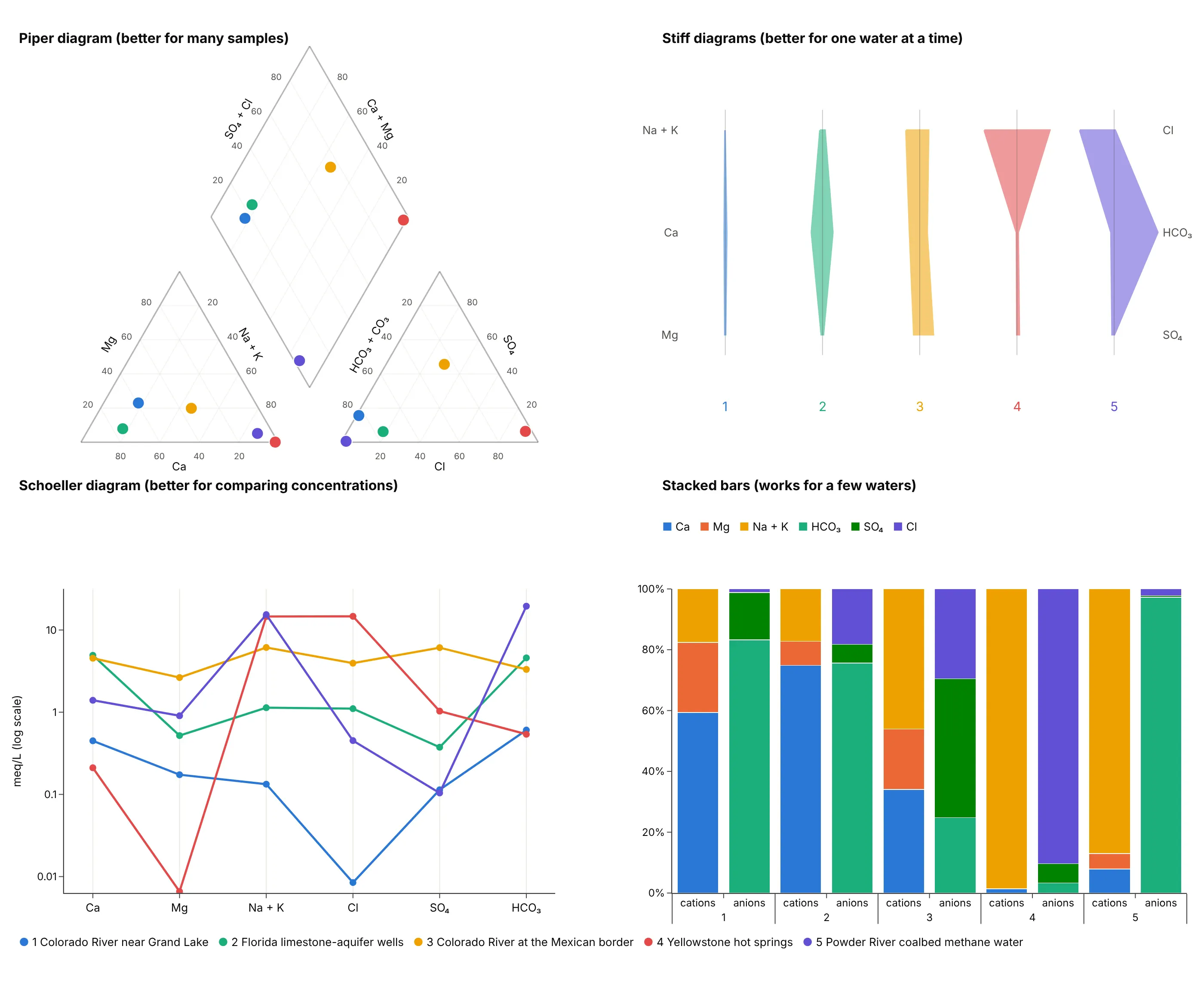
Five waters drawn four ways: a Piper diagram with five dots, five Stiff polygons growing from a sliver for Colorado River headwater to wide shapes for coalbed methane water, a Schoeller diagram with five lines on a log axis, and 100% stacked bars of cations and anions

Piper diagram (better for many samples). Hundreds or thousands of samples fit on one chart, and the diamond sorts them into water types, but a dot shows only proportions and not concentration.
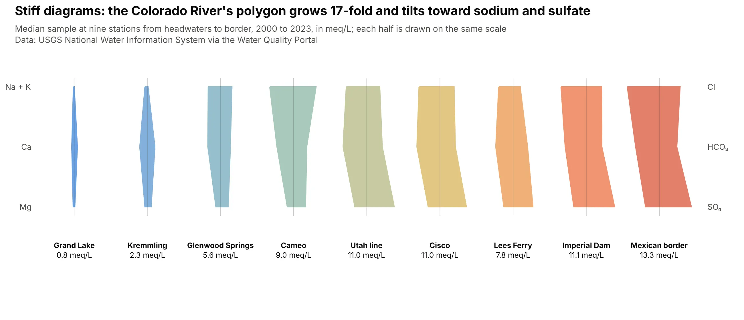
Stiff diagram (better for one water at a time). A polygon per sample, with cations on the left and anions on the right in meq/L, shows both the shape (the water type) and the size (the concentration), and polygons sit well on a map, but only a handful can be compared at once.
Schoeller diagram (better for comparing concentrations). One line per sample across the six ions on a log axis keeps the concentration and the pattern, so Colorado River water near its headwaters (0.8 meq/L of cations) and at the Mexican border (13.3 meq/L) can share an axis, but the lines tangle past a dozen samples.
Stacked bars (works for a few waters). Percent bars for cations and anions give the same proportions as the triangles and are easy to read, but they are one bar per sample and do not classify.
Ternary plots (works too, as the two triangles). The cation and anion panels of a Piper diagram are ternary plots, so if you only need one triangle the ternary guide covers it, but without the diamond you lose the combined water type.
Durov diagram (different). It draws the two triangles on the top and side of a square and adds panels for pH and total dissolved solids, so it carries two more variables than a Piper diagram. Example 3 below draws one.
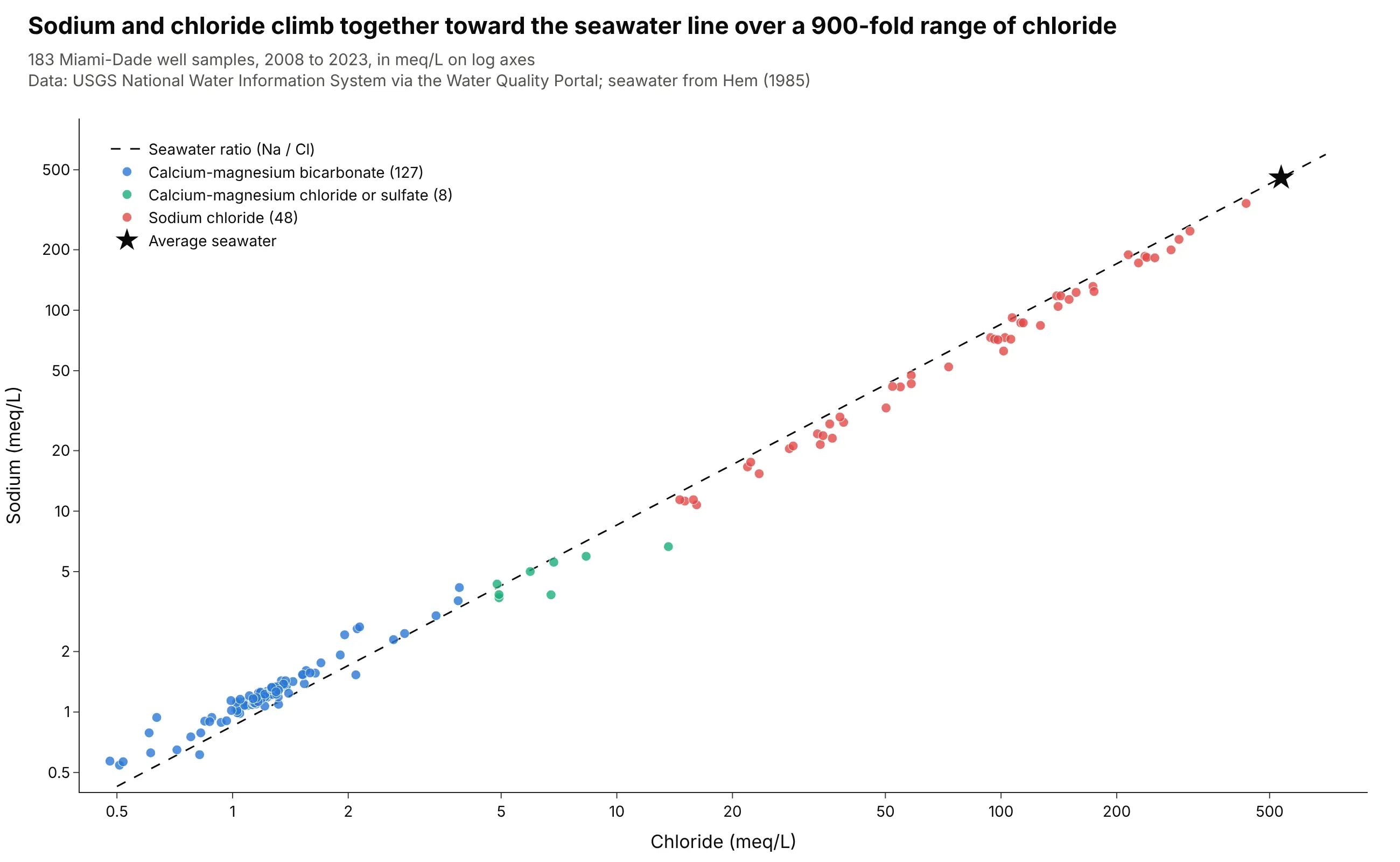
Scatter plot of two ions (better for a single process). Sodium against chloride on log axes keeps concentrations and shows mixing as a line, as the Miami-Dade wells below do.

Scatter plot of sodium against chloride in milliequivalents per liter on log axes for 183 Miami-Dade wells, with samples rising along a dashed seawater line from 0.5 meq/L to the seawater star at 536 meq/L

How to make a Piper diagram

With AI

ChatGPT, Claude Code, GitHub Copilot, Cursor and other AI tools are excellent at writing Plotly code. Name Plotly in the prompt, and say how to convert units and what to draw in the diamond:

Make a plotly Piper diagram from wells.csv (columns: site, date, ca, mg, na, k, cl, so4, alk_caco3 in mg/L).

- Convert mg/L to meq/L with equivalent weights (Ca 20.04, Mg 12.15, Na 22.99, K 39.10, Cl 35.45, SO4 48.03,
  HCO3 61.02; alkalinity as CaCO3 divided by 50.04) and drop samples whose charge balance error is above 10%.
- Draw the cation triangle at lower left, the anion triangle at lower right and the diamond above, on one pair
  of axes with equal scales, with 20% gridlines, tick labels and the dotted 50% lines in the diamond.
- Draw each sample as a dot in all three panels, colored by water type, with hover text showing the percents.
- Check: print how many samples were dropped and how many fall in each water type.

With Plotly Studio

Plotly Studio is a desktop app where you point an AI at a dataset and it builds charts and a Dash app around your questions. Ask for a Piper diagram the same way:

Show a Piper diagram of the groundwater samples in this file, converting the ions to milliequivalents per liter, with each sample colored by water type, a star for average seawater, and the sodium chloride samples listed in a table next to it.

Make a Piper diagram in Python or JavaScript

This is the code AI tools write under the hood. You can make a Piper diagram with Plotly from scatter points on one pair of axes with equal scales, with the triangle and diamond outlines drawn as lines, and the helper below does exactly that. The ternary plot guide covers Plotly's own ternary trace, which can draw the two triangles but not the diamond.

import numpy as np
import pandas as pd
import plotly.graph_objects as go

MG_PER_MEQ = dict(ca=20.04, mg=12.15, na=22.99, k=39.10, cl=35.45, so4=48.03, hco3=61.02)  # milligrams in one meq


def piper(df):
    """df has ca, mg, na, k, cl, so4 and hco3 in mg/L, one row per sample."""
    meq = pd.DataFrame({ion: df[ion] / w for ion, w in MG_PER_MEQ.items()})
    cat = meq[["ca", "mg", "na", "k"]].sum(axis=1)
    an = meq[["cl", "so4", "hco3"]].sum(axis=1)
    mg, nak = meq.mg / cat, (meq.na + meq.k) / cat       # share of cations
    so4, cl = meq.so4 / an, meq.cl / an                  # share of anions
    h, g = np.sqrt(3) / 2, 0.32                          # triangle height, gap between the triangles

    fig = go.Figure()
    outlines = [[(0, 0), (1, 0), (.5, h)],                                   # cations: Ca left, Na+K right, Mg top
                [(1 + g, 0), (2 + g, 0), (1.5 + g, h)],                      # anions: HCO3 left, Cl right, SO4 top
                [(1 + g / 2, h * g), (1.5 + g / 2, h * (1 + g)), (1 + g / 2, h * (2 + g)), (.5 + g / 2, h * (1 + g))]]
    for pts in outlines:
        fig.add_scatter(x=[p[0] for p in pts + pts[:1]], y=[p[1] for p in pts + pts[:1]], mode="lines",
                        line=dict(color="gray"), showlegend=False, hoverinfo="skip")
    fig.add_scatter(x=nak + mg / 2, y=h * mg, mode="markers", name="Cations")
    fig.add_scatter(x=1 + g + cl + so4 / 2, y=h * so4, mode="markers", name="Anions")
    fig.add_scatter(x=1 + g / 2 + (nak + so4 + cl - 1) / 2, y=h * (1 + g) + h * (so4 + cl - nak), mode="markers",
                    name="Diamond")
    fig.update_xaxes(visible=False)
    fig.update_yaxes(visible=False, scaleanchor="x")
    return fig.update_layout(template="simple_white", width=1000, height=800)


df = pd.read_csv("wells.csv")  # ca, mg, na, k, cl, so4, hco3 in mg/L
piper(df).show()

The function converts to meq/L, takes percents, and places each sample with the same barycentric formulas as a ternary plot: in the cation triangle the x position is Na + K plus half of Mg and the y position is Mg times the triangle height, and the diamond is placed by its Na + K and Cl + SO₄ shares. Adding gridlines, tick labels and the charge balance filter takes another 40 lines, which are in this guide's make_piper.py. In JavaScript, plotly.js draws the same thing from base traces:

<div id="chart"></div>
<script src="https://cdn.plot.ly/plotly-4.1.1.min.js"></script>
<script>
  // Median water of five groups, in milliequivalents per liter (ca, mg, na, k, cl, so4, hco3)
  const waters = {
    "Colorado River near Grand Lake": [0.45, 0.17, 0.10, 0.03, 0.01, 0.11, 0.61],
    "Florida limestone-aquifer wells": [4.93, 0.52, 1.09, 0.05, 1.10, 0.37, 4.59],
    "Colorado River at the Mexican border": [4.54, 2.64, 6.00, 0.13, 3.95, 6.10, 3.32],
    "Yellowstone hot springs": [0.21, 0.01, 13.96, 0.64, 14.70, 1.03, 0.54],
    "Powder River coalbed methane water": [1.40, 0.91, 15.14, 0.26, 0.45, 0.10, 19.50],
  };
  const h = Math.sqrt(3) / 2, g = 0.32;
  const outlines = [
    [[0, 0], [1, 0], [0.5, h]],                                       // cations: Ca left, Na+K right, Mg top
    [[1 + g, 0], [2 + g, 0], [1.5 + g, h]],                           // anions: HCO3 left, Cl right, SO4 top
    [[1 + g / 2, h * g], [1.5 + g / 2, h * (1 + g)], [1 + g / 2, h * (2 + g)], [0.5 + g / 2, h * (1 + g)]],
  ].map(p => ({type: "scatter", mode: "lines", x: [...p, p[0]].map(v => v[0]), y: [...p, p[0]].map(v => v[1]),
               line: {color: "gray"}, showlegend: false, hoverinfo: "skip"}));

  const points = Object.entries(waters).map(([name, [ca, mg, na, k, cl, so4, hco3]]) => {
    const cat = ca + mg + na + k, an = cl + so4 + hco3;
    const m = mg / cat, nak = (na + k) / cat, s = so4 / an, c = cl / an;
    return {type: "scatter", mode: "markers", name, marker: {size: 12}, legendgroup: name,
      x: [nak + m / 2, 1 + g + c + s / 2, 1 + g / 2 + (nak + s + c - 1) / 2],
      y: [h * m, h * s, h * (1 + g) + h * (s + c - nak)]};
  });

  Plotly.newPlot("chart", [...outlines, ...points], {
    width: 1000, height: 800,
    xaxis: {visible: false}, yaxis: {visible: false, scaleanchor: "x"},
    legend: {x: 0.99, y: 0.99, xanchor: "right"}
  });
</script>

Share it

Every Plotly chart has a Share chart button (the cloud icon in its toolbar) that uploads it to Plotly Cloud and gives you a link. Only you can see it until you change its visibility.

For a live app, put the chart in a Dash app and publish it with the Plotly Cloud CLI. Coding agents can run these commands for you:

pip install "dash[cloud]"
plotly user login
plotly app publish

If your data has to stay in your own cloud or data center, publish to Dash Enterprise instead.

Dos and don'ts

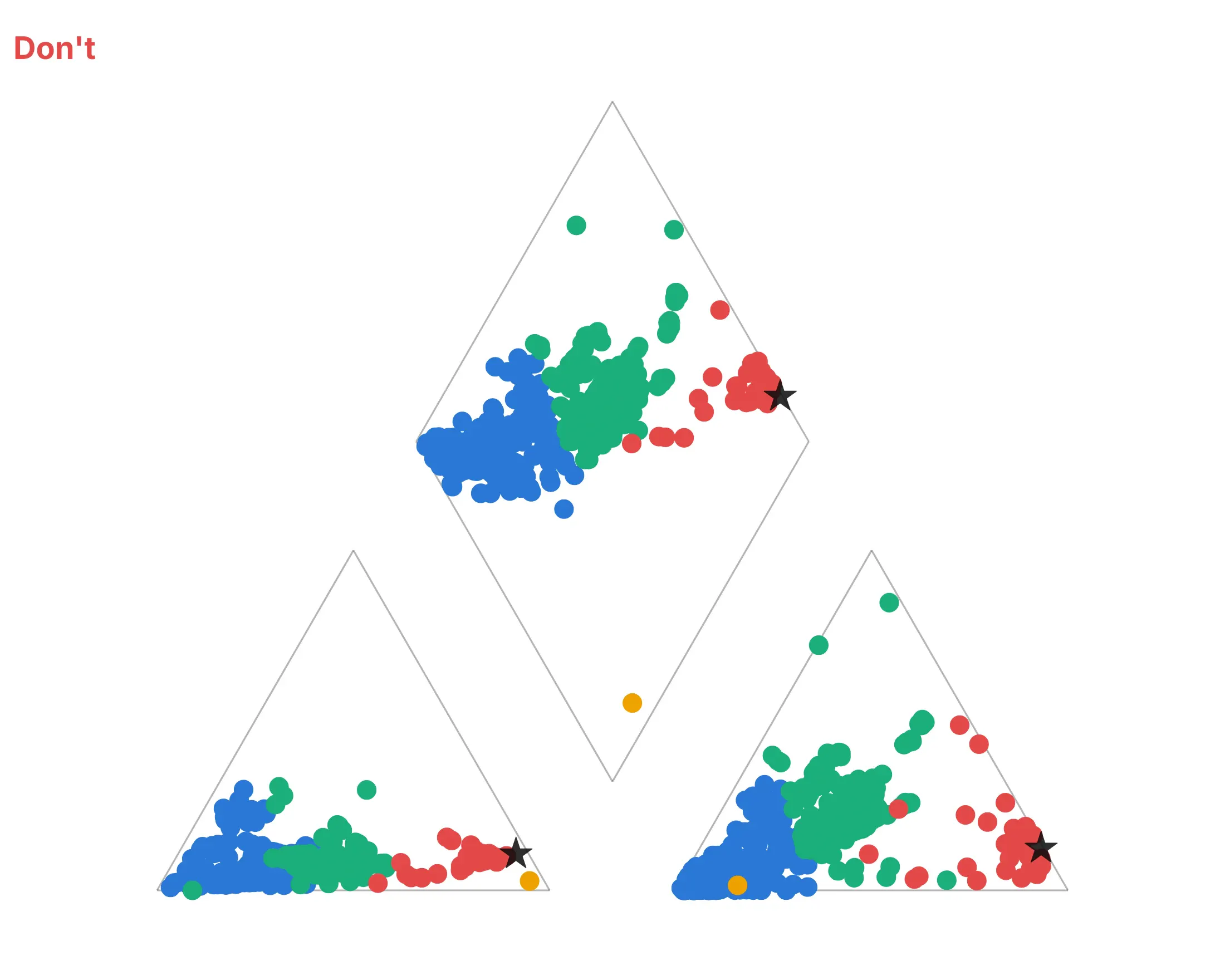
Most of the work in a published Piper diagram is the unit conversion and the frame around the dots. Here are the same 533 Florida samples both ways, in the same colors.

Don't compute percentages from mg/L instead of meq/L, draw large opaque markers that pile on top of each other, or leave out the gridlines, tick labels, axis titles, 50% lines, corner names and legend, so nobody can tell which corner or color is which:

The 533 Florida samples and the average-seawater star as large opaque dots in three empty outlines with no gridlines, ticks, axis titles, corner names or legend, and percentages computed from mass

Do convert to milliequivalents first, draw small partly transparent dots, add gridlines every 20%, tick labels, axis titles, the dotted 50% lines, the names of the four corners, a legend and a star for average seawater:

The same 533 samples with percentages from milliequivalents, small semi-transparent dots, 20% gridlines, tick labels, axis titles, dotted 50% lines, corner names, a star for average seawater and a legend with the number of samples per water type

Checklist

Convert mg/L to meq/L before taking percents, and drop samples with a charge balance error above about 10%.
Use equal scales on both axes, so the triangles are equilateral and the diamond is a true rhombus.
Color by water type or by a meaningful group, and add a reference such as average seawater.
Add circle size for total dissolved solids, or a second chart, when the amount matters.
Put the corner names and axis titles on the chart.

Don't

Take percents of mg/L.
Draw a Piper diagram of one sample (a Stiff diagram reads better) or of ions that are not major, such as nitrate or iron.
Read concentration into the position of a point, because only proportions are plotted.
Treat a point near a 50% line as clearly one type or the other.

Options to customize

A Piper diagram in Plotly is a set of go.Scatter traces plus layout settings, so these are the options that matter most. The full lists are in the scatter trace reference and the layout reference.

yaxis.scaleanchor="x": locks the two axes to equal scales so the triangles stay equilateral; add constrain="domain" to keep the plot area inside its box.
go.Scatter(mode="lines") or layout shapes: draws the outlines, gridlines and 50% lines. Shapes with layer="below" keep them behind the dots.
marker.size with an array: sizes each dot by a column such as total dissolved solids; use the square root of the value so the area follows it.
marker.opacity, marker.line: partly transparent dots with a thin white outline keep dense clusters readable.
legendgroup and showlegend=False on two of the three traces: one legend entry per group that toggles all three panels together.
hovertext, hoverinfo="text": the site name and the six percents on hover.
marker.color with marker.coloraxis: colors the dots by a number such as streamflow, with one shared colorbar.
annotations: tick labels, axis titles and corner names, with textangle to run titles along the triangle edges.
go.Scattergl: WebGL points for tens of thousands of samples; the benchmark in the FAQ shows the difference.
mode="markers+text", textposition: labels on the few points the story needs, such as one dot per river.
template="simple_white", width, height: a white background and a fixed size, so the equal-scale frame does not stretch.

More Piper diagram examples

Seven more Piper diagrams built from real water analyses, each with its source, a tip and a prompt to rebuild it.

1. The Colorado River from the headwaters to the Mexican border

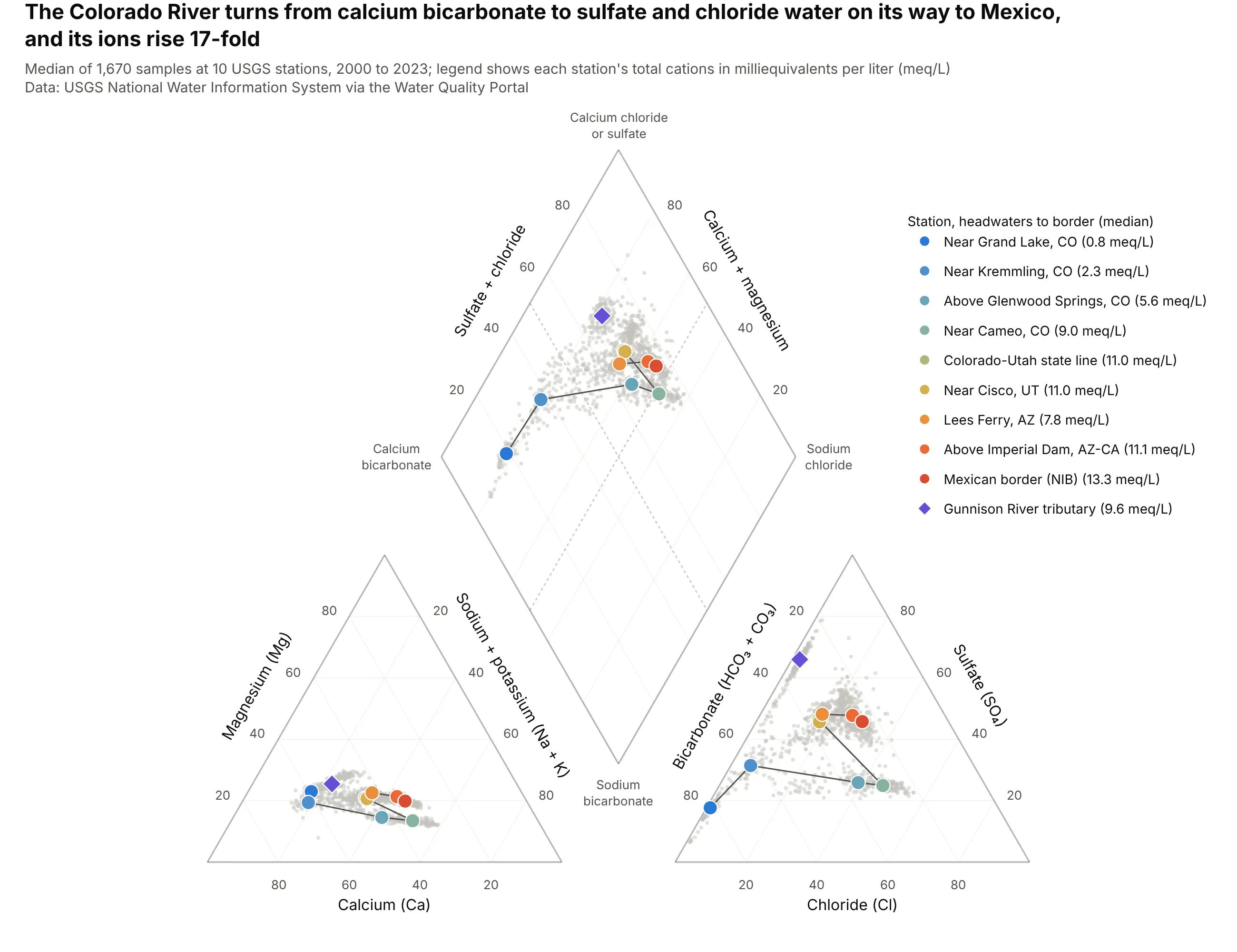
Piper diagram of Colorado River samples at 10 stations, gray dots for every sample and large dots for the station medians from blue near Grand Lake to orange at the Mexican border joined by a line, moving from the calcium bicarbonate corner toward the middle of the diamond, with the Gunnison River as a purple diamond

The median sample near Grand Lake holds 0.8 meq/L of cations, 60% of them calcium, and the one at the Mexican border holds 13.3 meq/L, a 17-fold rise, with sulfate (46%) and chloride (30%) taking over from bicarbonate. The Gunnison River tributary has a median of 66% sulfate. Data: USGS NWIS via the Water Quality Portal, 10 stations, 2000 to 2023.

Tip: join the station medians in river order, and draw every sample in light gray behind them, so the path is the story and the spread is still visible.

Another way to see it: Stiff diagrams of the nine main-stem stations grow from a sliver at Grand Lake to a wide, tilted shape at the border.

Nine Stiff diagrams of the Colorado River's median water from Grand Lake at 0.8 meq/L to the Mexican border at 13.3 meq/L, widening and tilting from calcium bicarbonate toward sodium and sulfate

Get the data from the USGS Water Quality Portal (waterqualitydata.us, NWIS provider), samples at USGS sites
09011000, 09058000, 09071750, 09095500, 09152500, 09163500, 09180500, 09380000, 09429490 and 09522000 since
2000, and shape it into a table (columns: site, date, ca, mg, na, k, cl, so4, alk in mg/L).

Build a plotly Piper diagram from the data: convert to meq/L, drop samples with charge balance error above
10%, draw every sample in light gray, the median of each station as a large dot from blue to orange in river
order joined by a line, and the Gunnison River as a purple diamond.

2. One station, 24 years: the Colorado River near Cameo

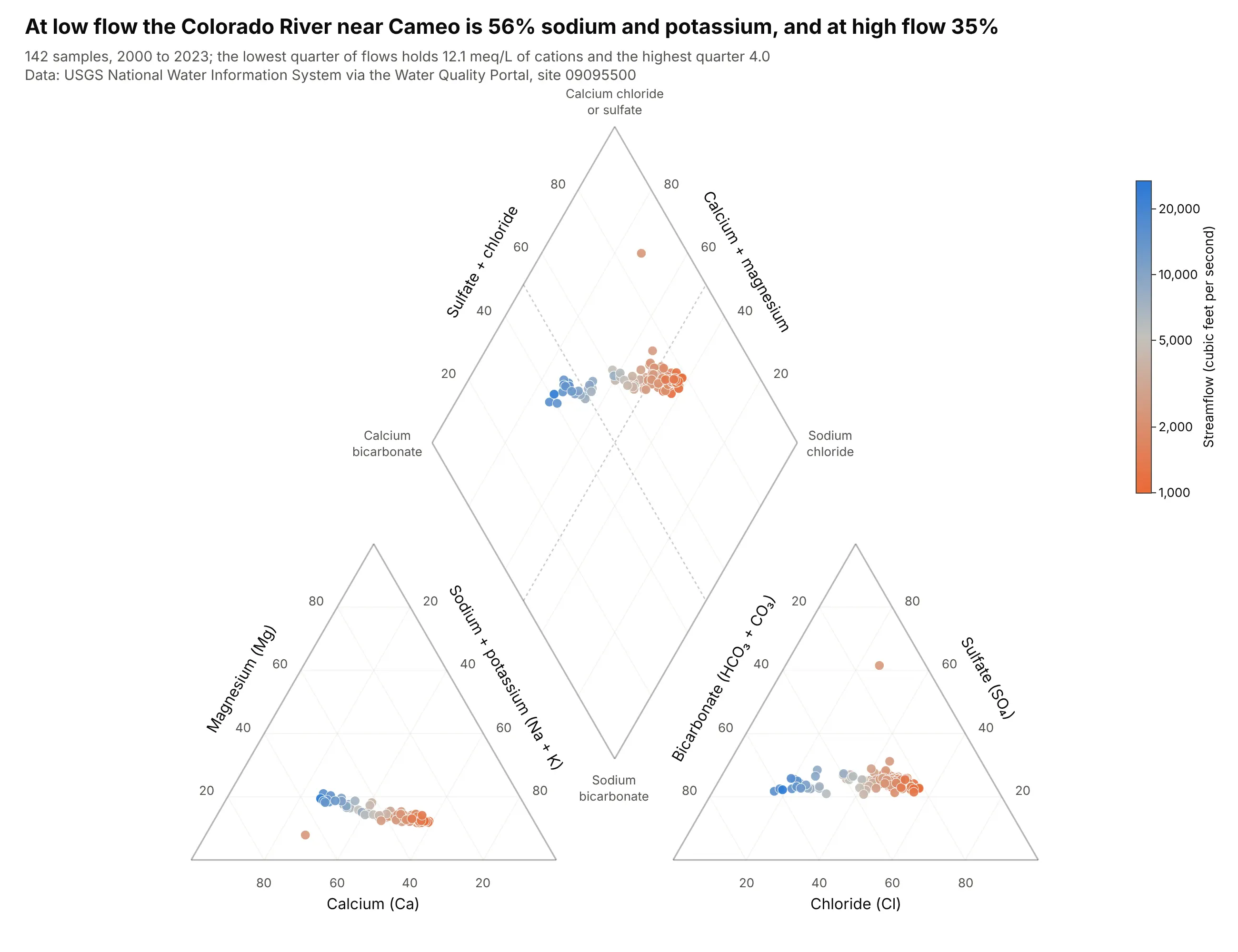
Piper diagram of 142 samples from the Colorado River near Cameo, Colorado, colored by streamflow from orange at 1,000 cubic feet per second to blue at 26,000, with orange dots at the sodium chloride side and blue dots at the calcium bicarbonate side

At low flows (the lowest quarter, up to 1,700 cubic feet per second) the median sample is 56% sodium plus potassium with 12.1 meq/L of cations, and at high flows (above 3,135) it is 35% and 4.0 meq/L. Flow and total cations have a rank correlation of -0.95 across the 142 samples. Data: USGS NWIS via the Water Quality Portal, site 09095500, 2000 to 2023.

Tip: color the dots by a continuous variable such as streamflow on a log scale, and use one shared colorbar through marker.coloraxis.

Get the data from the USGS Water Quality Portal (NWIS) for site USGS-09095500, Colorado River near Cameo,
Colorado, since 2000: major ions plus the instantaneous streamflow on each sample date, and shape it into a
table (columns: date, ca, mg, na, k, cl, so4, alk in mg/L, flow_cfs).

Build a plotly Piper diagram: convert to meq/L, color each sample by log10 of streamflow with a single colorbar
in cubic feet per second, and put the quartile medians of sodium plus potassium in the title.

3. Hot springs and cold springs in Yellowstone

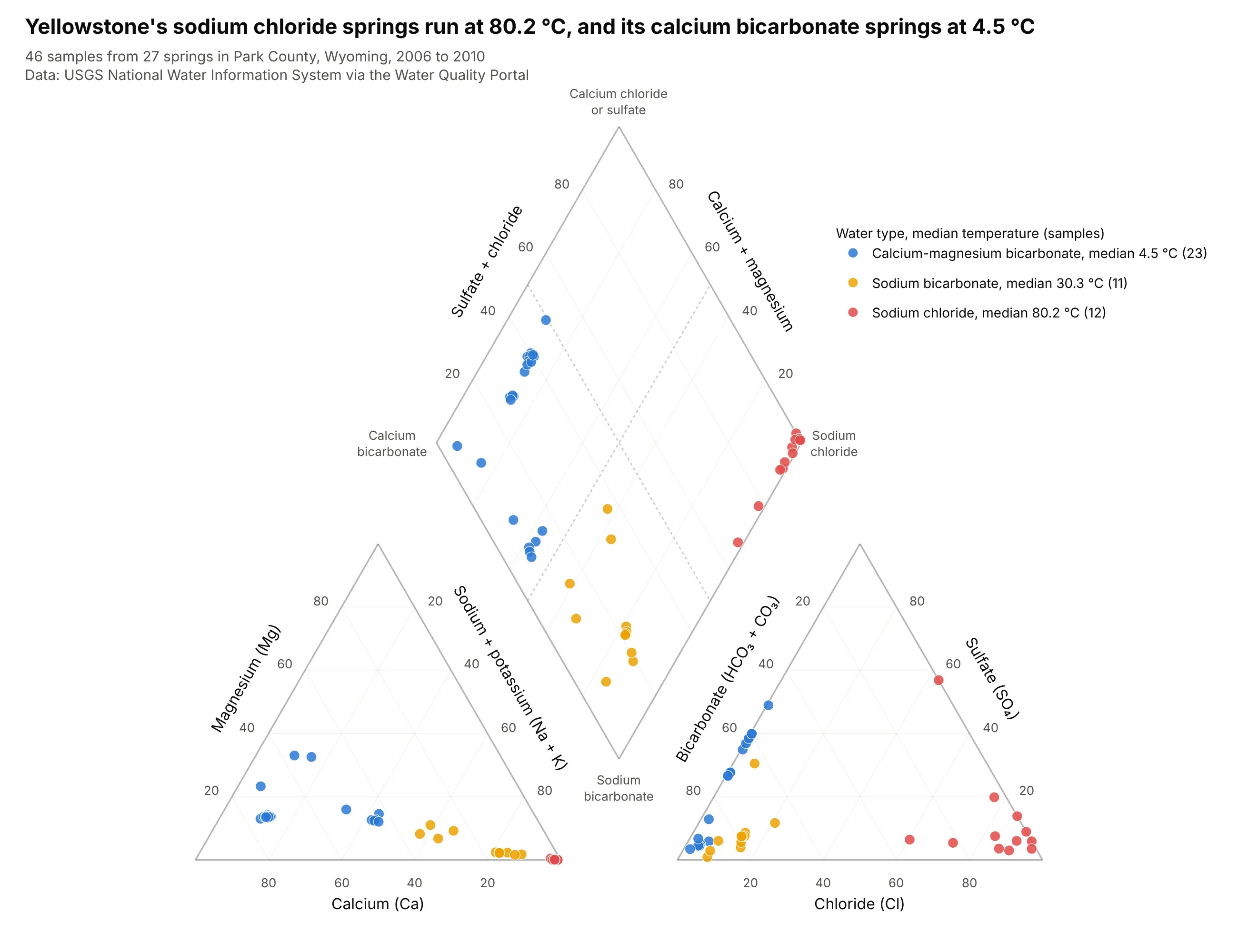
Piper diagram of 46 Yellowstone spring samples: 23 calcium-magnesium bicarbonate in blue at the left corner, 11 sodium bicarbonate in yellow near the bottom corner and 12 sodium chloride in red at the right corner

The 12 sodium chloride samples come from springs with a median temperature of 80.2 °C, the 11 sodium bicarbonate samples from springs at 30.3 °C, and the 23 calcium-magnesium bicarbonate samples from springs at 4.5 °C. The type separates cleanly by temperature across 46 samples from 27 springs. Data: USGS NWIS via the Water Quality Portal, Park County, Wyoming, 2006 to 2010.

Tip: two acidic samples (pH 3.4 and 3.6) have no alkalinity at all, so their bicarbonate share is 0%; for water below pH 4.5 a Piper diagram reads sulfate and chloride only, and a note on the chart saves questions.

Another way to see it: a Durov diagram adds the pH and total ions of each sample in two side panels, and shows that the hot chloride springs span pH 3.4 to 7.7.

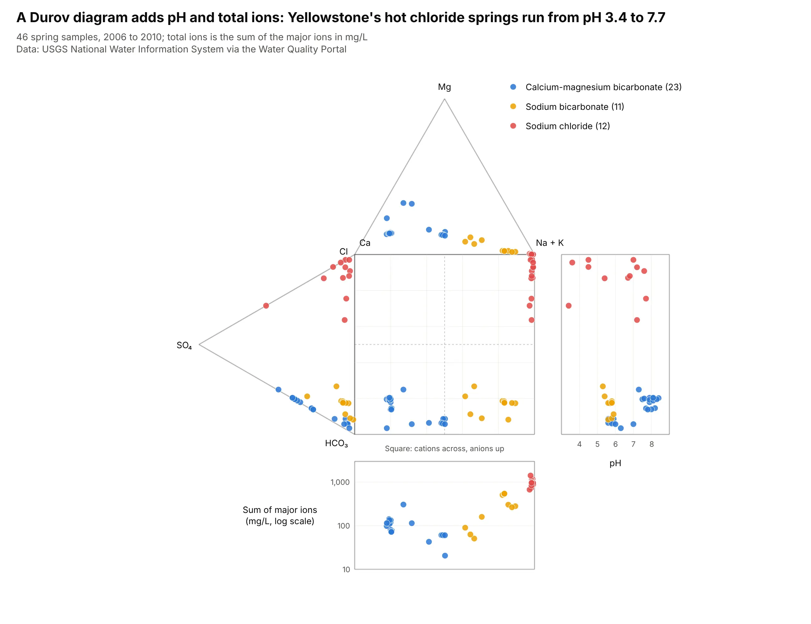
Durov diagram of 46 Yellowstone spring samples: a cation triangle above and an anion triangle at the left of a square, with panels for pH to the right and the sum of the major ions below

Get the data from the USGS Water Quality Portal (NWIS) for springs in Park County, Wyoming (state US:56,
county 029) since 2000: major ions plus water temperature and pH, and shape it into a table (columns: site,
name, date, ca, mg, na, k, cl, so4, alk in mg/L, temp_c, ph).

Build a plotly Piper diagram: convert to meq/L, color samples by water type, and put each type's median
temperature in the legend.

4. Sixteen large US rivers, one dot each

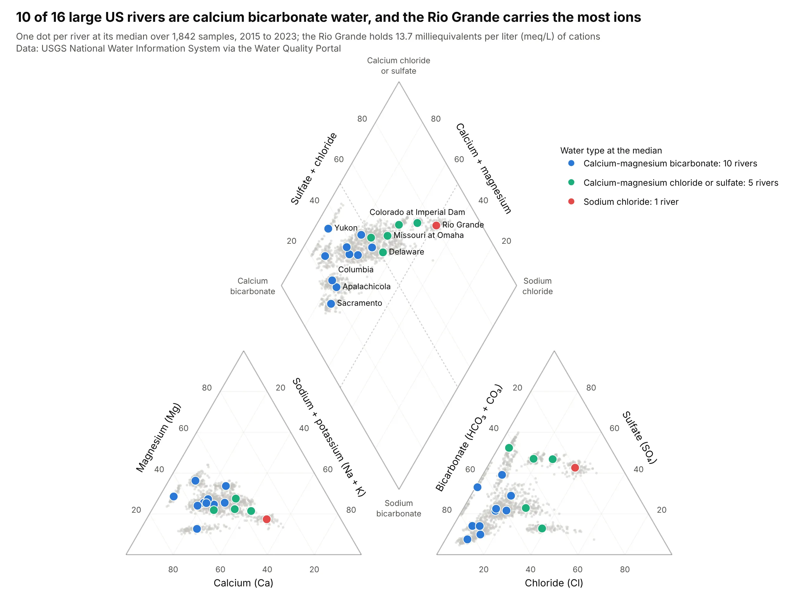
Piper diagram of 16 large US rivers, one dot per river at its median over 1,842 samples: 10 blue calcium bicarbonate rivers near the left corner, 5 green calcium chloride or sulfate rivers in the middle and the Rio Grande in red as the only sodium chloride river

At the median, 10 of the 16 rivers are calcium-magnesium bicarbonate water, 5 are calcium-magnesium chloride or sulfate and only the Rio Grande is sodium chloride. It also carries the most dissolved cations, 13.7 meq/L, against 1.2 meq/L for the Apalachicola. Data: USGS NWIS via the Water Quality Portal, 16 stations, 2015 to 2023.

Tip: with 1,842 samples, draw them in light gray and put one labeled dot on each river's median, so the chart reads as 16 names and not as a cloud.

Get the data from the USGS Water Quality Portal (NWIS) for 16 river sites (Columbia 14246900, Sacramento
11447650, Yukon 15565447, Upper Mississippi 05420500, Lower Mississippi 07373420, Atchafalaya 07381495, Missouri
06610000 and 06934500, Ohio 03303280 and 03612600, Susquehanna 01578310, Delaware 01463500, Apalachicola 02359170,
Colorado 09380000 and 09429490, Rio Grande 08475000) since 2015, and shape it into a table (columns: site, river,
date, ca, mg, na, k, cl, so4, alk in mg/L).

Build a plotly Piper diagram: every sample in light gray, one large colored dot per river at the median colored by
water type, and label the dots for the Yukon, Columbia, Delaware, Missouri at Omaha, Colorado and Rio Grande.

5. Great Salt Lake and Walker Lake

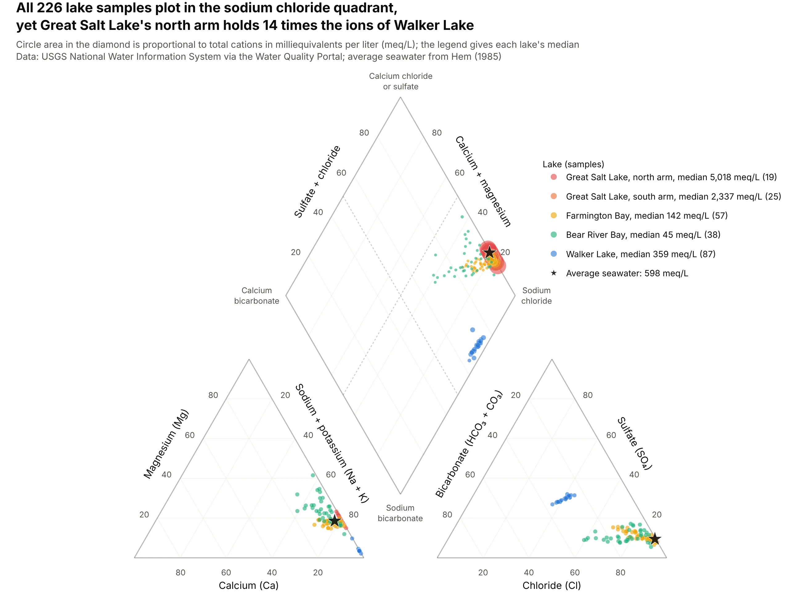
Piper diagram of 226 lake samples all in the sodium chloride quadrant, with circles in the diamond sized by total cations: very large for Great Salt Lake's north arm at 5,018 meq/L, small for Bear River Bay at 45 meq/L, and a black star for seawater at 598 meq/L

All 226 samples plot in the sodium chloride quadrant, yet the north arm of Great Salt Lake holds a median of 5,018 meq/L of cations, 14 times Walker Lake's 359 and 8.4 times seawater's 598. Circle area in the diamond restores what percentages hide. Data: USGS NWIS via the Water Quality Portal, 7 sites, 2012 to 2023.

Tip: size the diamond circles by the square root of the concentration so that area, and not diameter, follows the value, and cap the largest one so it does not cover the others.

Get the data from the USGS Water Quality Portal (NWIS) for Great Salt Lake (sites 10010026, 10010025,
410401112134801 and 10010060) and Walker Lake (384506118433001, 383903118425301 and 384200118431901) since 2012,
and shape it into a table (columns: site, lake, date, ca, mg, na, k, cl, so4, alk in mg/L).

Build a plotly Piper diagram: convert to meq/L, one color per lake, diamond circle area proportional to total
cations, and a star for average seawater (598 meq/L).

6. Albuquerque's aquifer, deeper and saltier in chloride

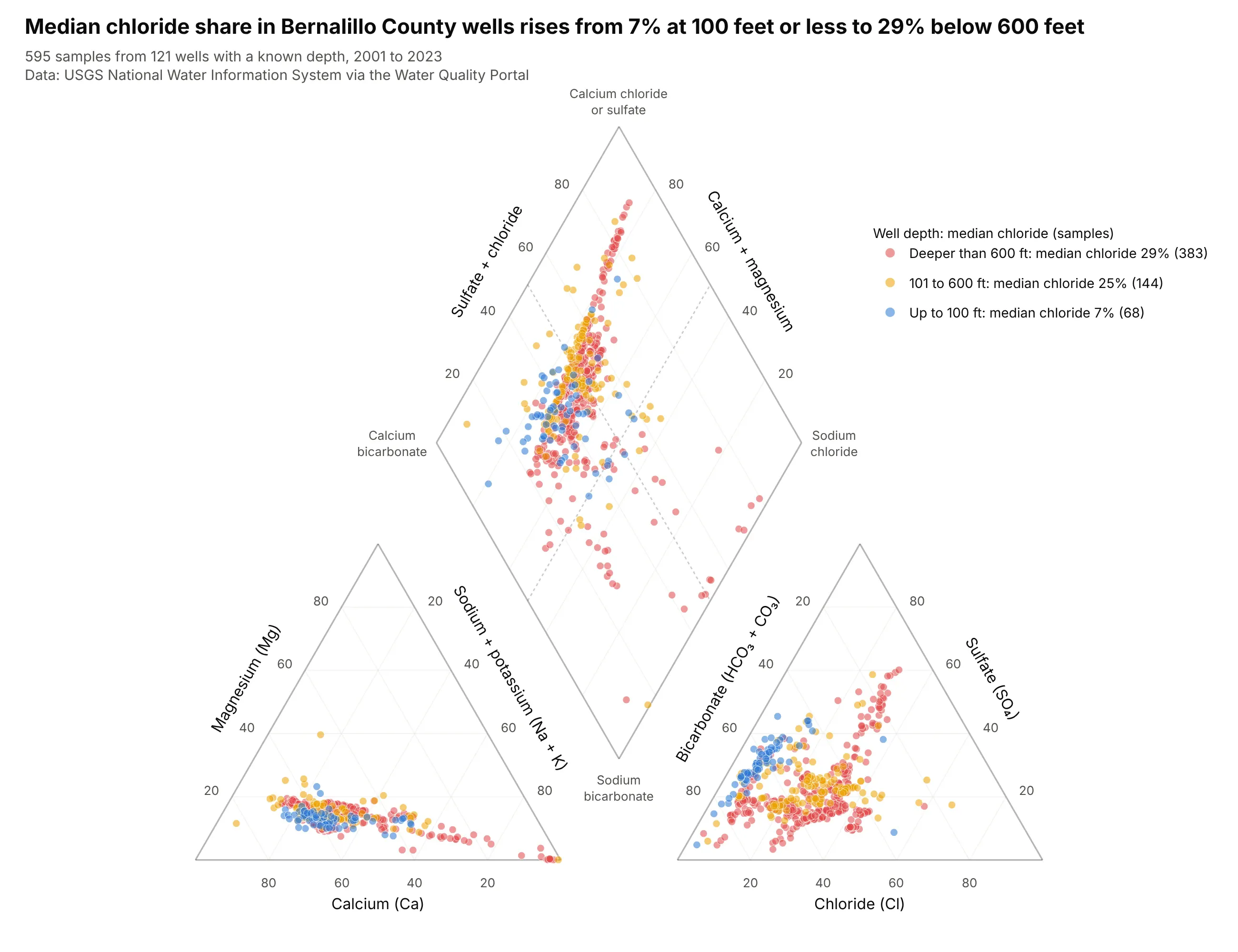
Piper diagram of 595 well samples in Bernalillo County, New Mexico, colored by well depth: blue dots for wells up to 100 feet deep cluster at the calcium bicarbonate corner, while yellow and red dots for deeper wells spread toward the chloride and sulfate side

The median chloride share of the anions rises from 7% in wells up to 100 feet deep to 25% between 101 and 600 feet and 29% below 600 feet, and 81% of the shallowest samples are calcium-magnesium bicarbonate against 54% of the deepest. The county is the one Chris Parmer's Compendium of Canonical Charts uses for its Piper diagram. Data: USGS NWIS via the Water Quality Portal, Bernalillo County, New Mexico, 595 samples from 121 wells with a known depth, 2001 to 2023.

Tip: draw the groups from the largest to the smallest, so the 68 shallow samples sit on top of the 383 deep ones instead of under them.

Get the data from the USGS Water Quality Portal (NWIS) for wells in Bernalillo County, New Mexico (state US:35,
county 001) since 2000: major ions, plus each well's depth in feet from the Station service, and shape it into a
table (columns: site, date, ca, mg, na, k, cl, so4, alk in mg/L, well_depth).

Build a plotly Piper diagram: convert to meq/L, color samples by well depth (up to 100 ft, 101 to 600 ft, deeper
than 600 ft) with the deepest group drawn first, and show each group's median chloride share in the legend.

7. Six kinds of water on one diamond

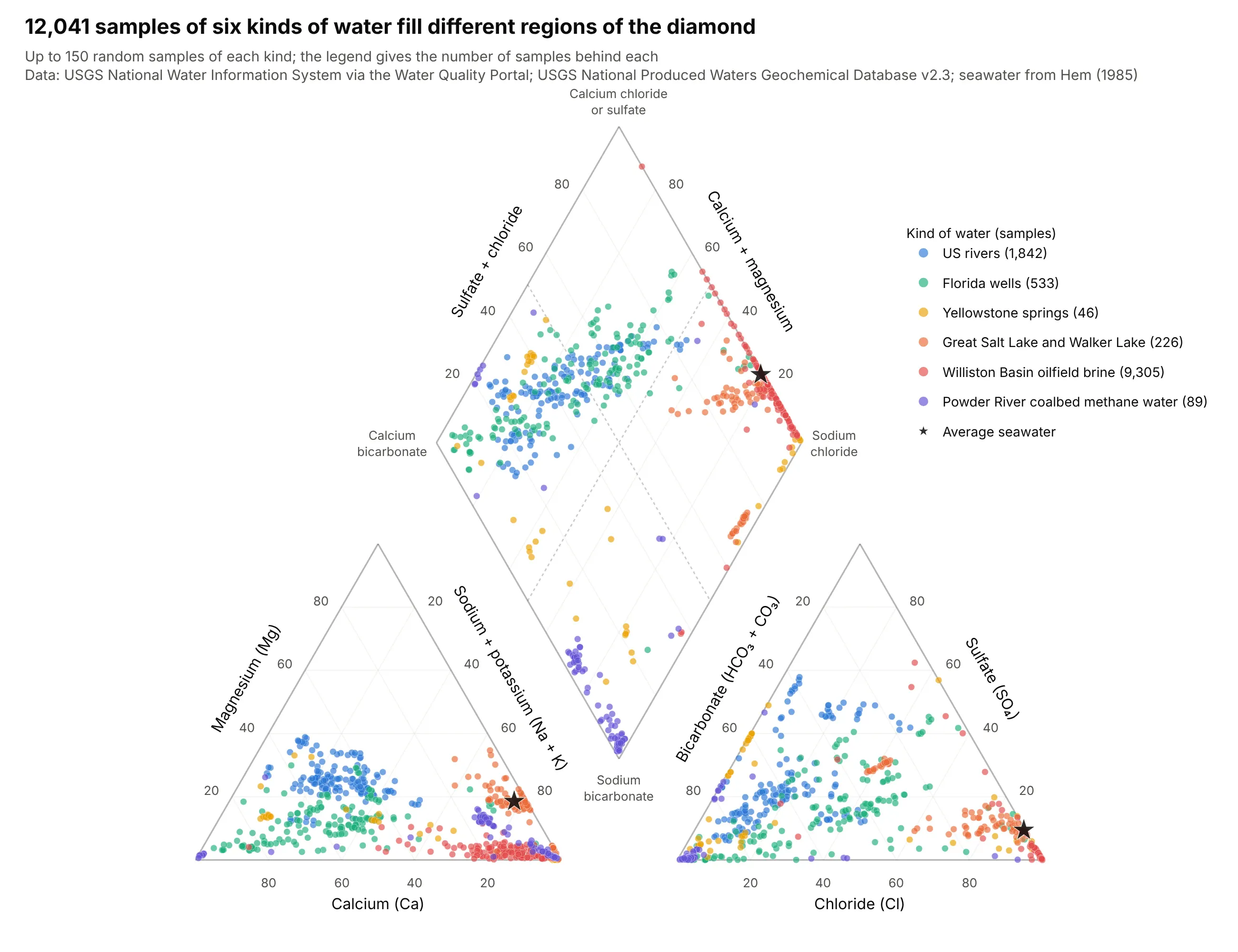
Piper diagram of up to 150 samples each from US rivers, Florida wells, Yellowstone springs, two saline lakes, Williston Basin oilfield brine and Powder River coalbed methane water, each kind in its own region of the diamond

Rivers and Florida wells fill the left half of the diamond, Yellowstone's springs run along its left and bottom edges, and the lakes and Williston brine crowd the sodium chloride corner at the right. The chart draws 150 of the 12,041 samples behind it for each kind of water. Data: USGS NWIS via the Water Quality Portal and USGS National Produced Waters Geochemical Database v2.3.

Tip: sample each kind to the same number of dots, with a fixed random seed, so a dataset with 9,305 samples does not bury one with 46.

Get the data from the USGS Water Quality Portal (NWIS) for the US rivers, Florida wells, Yellowstone springs and
saline lakes above, and from the USGS National Produced Waters Geochemical Database v2.3 (ScienceBase item
59d25d63e4b05fe04cc235f9) for Williston Basin conventional wells and Powder River Basin coalbed methane wells, and
shape them into one table (columns: kind, ca, mg, na, k, cl, so4, hco3 in mg/L).

Build a plotly Piper diagram: convert to meq/L, drop samples with charge balance error above 10%, draw 150 random
samples (seed 0) from each kind in its own color, and a star for average seawater.

Piper Diagrams - A Complete Guide

What is a Piper diagram?

A short history

Milliequivalents and percent, explained

Hydrochemical facies

Alternatives to a Piper diagram

How to make a Piper diagram

With AI

With Plotly Studio

Make a Piper diagram in Python or JavaScript

Share it

Dos and don'ts

Checklist

Options to customize

More Piper diagram examples

1. The Colorado River from the headwaters to the Mexican border

2. One station, 24 years: the Colorado River near Cameo

3. Hot springs and cold springs in Yellowstone

4. Sixteen large US rivers, one dot each

5. Great Salt Lake and Walker Lake

6. Albuquerque's aquifer, deeper and saltier in chloride

7. Six kinds of water on one diamond

FAQ

What is a Piper diagram?

How do you read a Piper diagram?

Is a Piper plot the same as a Piper diagram or a trilinear diagram?

What are hydrochemical facies?

How do I make a Piper diagram in Python?

What is the difference between a Piper diagram, a Stiff diagram and a Durov diagram?

Why does the Piper diagram use milliequivalents and not mg/L?

How many samples can a Piper diagram show?

Does a Piper diagram show how salty the water is?