What's new in Polars 2.0, tested in Dash apps on a billion rows

TL;DR

• Polars 2.0 came out on October 6, 2026. For Dash developers, the headline change is that collect() now runs on the streaming engine, which reads data in batches and can spill to disk. It also adds a Map type, much more SQL (including ROLLUP and APPROX_QUANTILE) and new binning functions.
• We built a four-page Dash app on 1.14 billion NOAA weather readings and 4.7 million Overture Maps places to try them out. Pulling one weather station's 57,634 days out of all 1.14 billion rows takes about 0.12 seconds.
• With default settings on a 16 GB machine, Polars 2.0 rolled all 1.14 billion rows up to months in 27 seconds using 4.8 GB. Polars 1.44 ran out of memory on the same job even with its streaming engine turned on, and its default engine ran out on five of our eight large tasks.
• Everything we tested ran as fast or faster in 2.0, with one exception: joins. On our biggest join, 2.0 needed more memory than 1.44's streaming engine, and out-of-core joins are still on Polars' roadmap.
• We list eight things that tripped us up, from joins that no longer keep row order to Map columns that SQL can't read yet. Most removed APIs fail with an error that names the replacement.

Why Polars matters for Dash apps

Polars is a DataFrame library for Python, written in Rust. Ritchie Vink created it, and it now has more than 40,000 stars on GitHub. Its lazy API lets you describe a whole query (scan these files, filter, join, group) before any data is read, so Polars can plan the work, skip the columns and row groups it doesn't need, and spread the rest across every core.

Dash, Plotly's Python framework for data apps, is a small web server where each chart is filled by a Python callback. The most common way to write those callbacks is still to load a pandas DataFrame when the app starts and filter it on every click. That works until the data gets big, and then every gunicorn worker holds its own full copy in memory. Polars fits the other pattern much better. You define a LazyFrame over Parquet files at the top of the app, which reads nothing, and each callback adds a filter and calls collect(). Plotly Express has accepted Polars DataFrames directly since plotly.py 6.0, so the result goes straight into a chart.

Polars 2.0 came out on October 6, 2026, after a release candidate in September. The Polars team calls it a deliberately "boring" release. It removes old APIs that held the library back and changes several defaults, and the biggest of those is that collect() now runs on the streaming engine. Streaming means Polars reads and processes data in batches instead of loading it all first, and in 2.0 it can also spill to disk when memory runs low. For a Dash app, where several worker processes share one machine, streaming makes a huge difference to memory use. A per-station summary of 119 million rows peaked at 9.2 GB on Polars 1.44's default engine and 1.4 GB on 2.0.

We built a four-page Dash app on two public datasets to try 2.0 out, and ran the same queries on Polars 1.44 and 2.0 on the same machine.

The first dataset is NOAA's GHCN-Daily, every daily weather reading NOAA has collected since 1763: 1.14 billion rows from 132,779 weather stations, stored as 1.8 GB of Parquet. It's the same data we used for our DuckDB 2.0 post, which makes the two posts easy to compare.

The second is Overture Maps, an open map dataset backed by Amazon, Meta, Microsoft and others. Its divisions layer lists 4.7 million countries, regions, cities and neighbourhoods, each with its name in as many languages as anyone has recorded.

Each chart in the app shows a small ⚡ badge with the time its Polars query took. All of those timings, and the benchmarks, come from a general-purpose Linux cloud VM with 4 vCPUs and 16 GB of RAM (not a Plotly Cloud app).

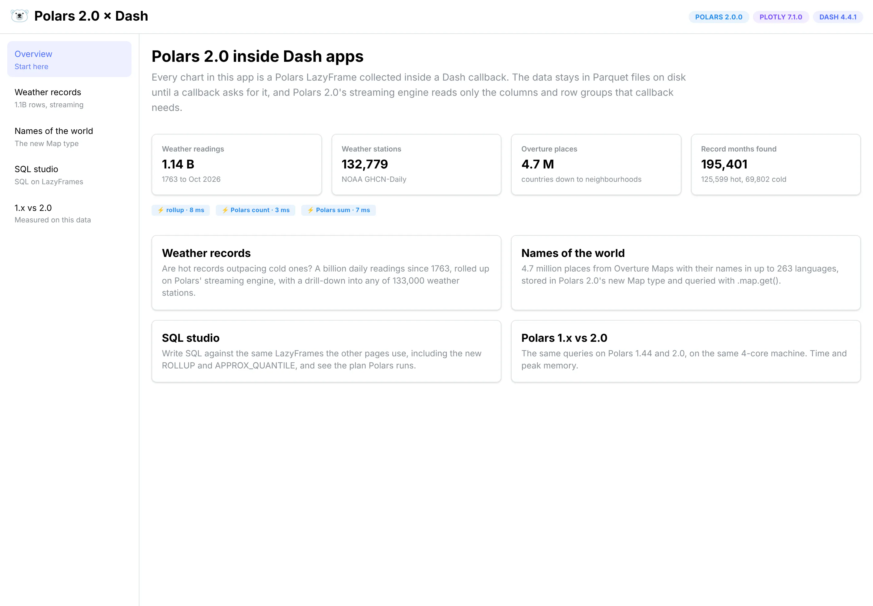
The overview page. Every number on it comes from a Polars query.

Weather records: a billion rows on the streaming engine

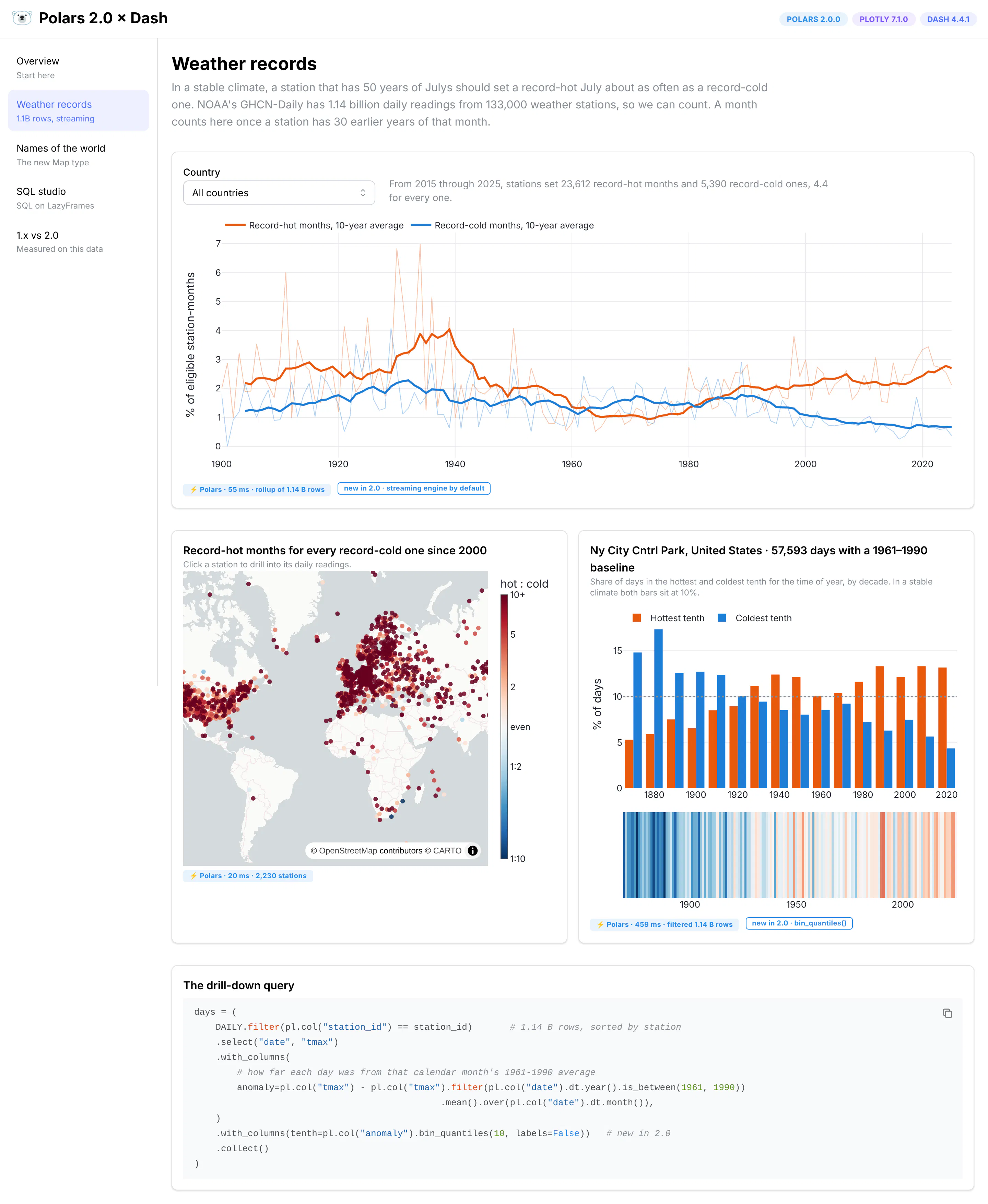
Record-hot and record-cold months as a share of all station-months that could have set one, 1900 to 2025. Clicking a station on the map queries its daily readings from the 1.14-billion-row table.

Overview of this app

• A chart of how often weather stations set a record-hot month compared with a record-cold one, by year, for any country
• A map of every station with a long enough record, colored by its ratio of hot records to cold ones since 2000
• Click a station to see how often its days land in the hottest or coldest tenth for the time of year, by decade, plus warming stripes

In a stable climate, a station with 50 years of Julys should set a record-hot July about as often as a record-cold one. That's roughly what happened from the late 1950s to the 1980s. Since then the two lines have pulled apart. From 2015 through 2025, stations in GHCN set 23,612 record-hot months and 5,390 record-cold ones, about 4.4 for every one. The 1930s stand out too, mostly from the United States, where the Dust Bowl summers still hold many records.

Polars 2.0 features

The streaming engine is the default. Nothing in this page asks for it. The scheduled job that builds the rollups is plain Polars code, and sink_parquet and collect() run on the streaming engine because that's what 2.0 does now:

That turns 1.14 billion daily rows into 39 million station-months in about 34 seconds. A second step finds the records with a window function: cum_max() over each station and calendar month, ordered by year, gives the record so far, and shift(1) compares each month with the record before it.

bin_quantiles() for the drill-down. 2.0 deprecates cut() and qcut() in favor of three new binning functions, bin_intervals(), bin_quantiles() and bin_ranks(). The station chart uses bin_quantiles(10) to put every day into a tenth of the station's distribution, after subtracting that calendar month's 1961 to 1990 average so that summer days don't fill the top tenth:

The query filters all 1.14 billion rows and comes back in 0.4 to 0.5 seconds, including the binning. In New York's Central Park, 12.8% of days since 2000 fell in the hottest tenth for their time of year and 6.0% in the coldest, where a stable climate would put 10% in each.

A few nice patterns

• Aggregate first, then window. Our first attempt ran the record-finding window directly on the daily table, with one window per station and calendar day. On a single year of data that's 12 million groups of one row each, and it took 48 seconds. Rolling up to months first made the window run on 39 million rows in 1.5 million groups, and the whole records step takes about 8 seconds.
• Sort Parquet by the column people filter on. Each yearly file is sorted by station_id, so Polars can skip almost every row group when a callback asks for one station. Reading one station's 57,634 days from all 264 files takes about 0.12 seconds.
• Sort before you draw a line. group_by doesn't promise any order, in 1.x or 2.0, so every chart that draws lines sorts by year first.

Names of the world: the new key-value Map type

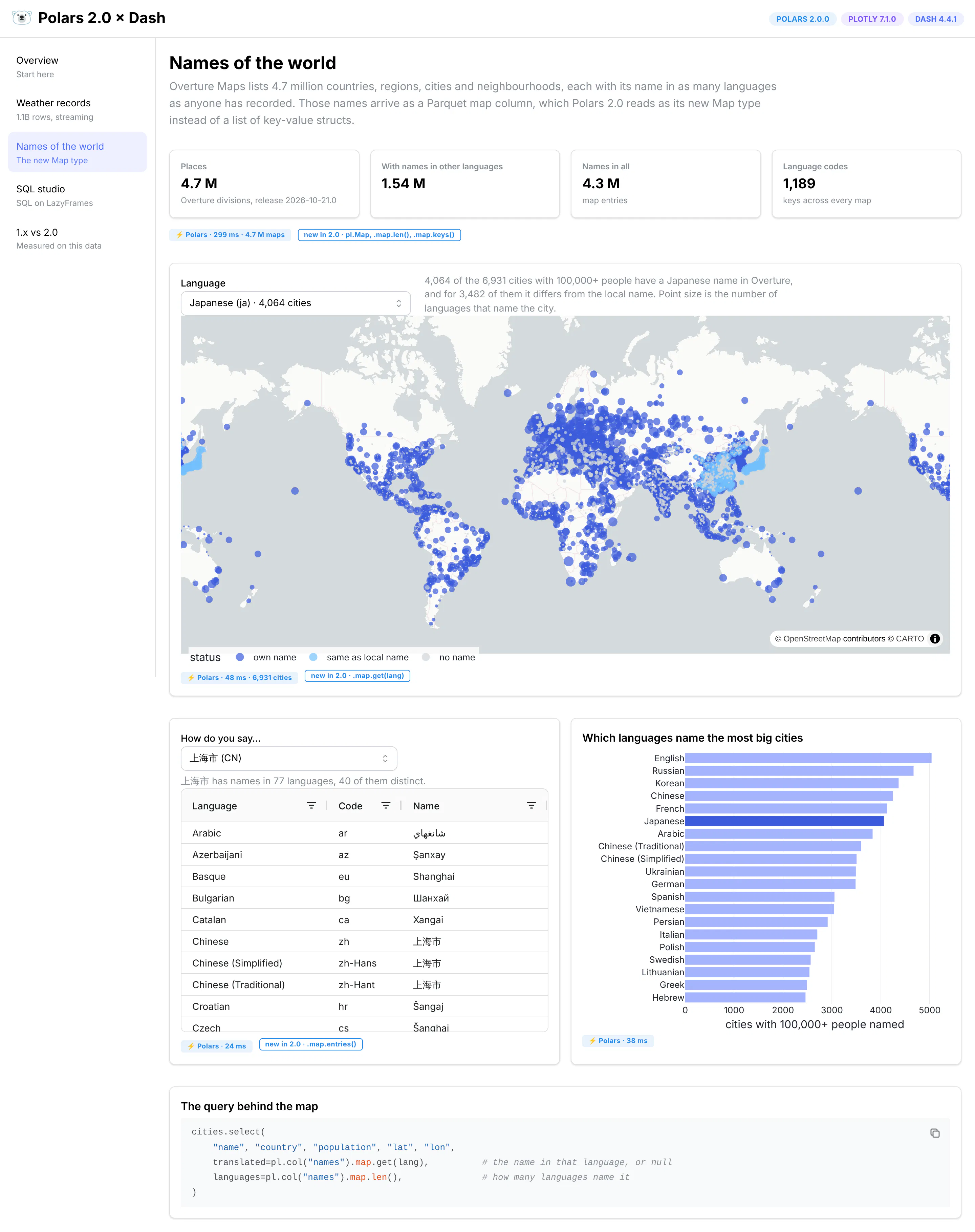
Every city with 100,000 or more people, colored by whether Overture has a Japanese name for it. Below, Shanghai's 77 names and the languages that name the most big cities.

Overview of this app

• Pick a language and see which of the world's 6,931 cities with 100,000 or more people have a name in it, and where that name differs from the local one
• Pick a city and see every name it has, in every language
• A chart of which languages name the most big cities

Some of this is fun to browse. London has names in 263 languages, more than any other city in Overture, although countries go higher (Afghanistan has 301). 4,064 of the big cities have a Japanese name, and for 3,482 of them it differs from the local name. Shanghai has 77 names, but only 40 distinct ones, because many languages write it as 上海市 or Shanghai.

Polars 2.0 features

The Map dtype. Despite the name, this has nothing to do with geographic maps. A Map column holds a set of key-value pairs in every row, much like a Python dictionary. Overture stores each place's names this way, with the language code as the key and the name as the value, so London's row holds {"fr": "Londres", "de": "London", "ja": "ロンドン", ...} and 260 more entries. Different rows have different keys, which is why a column per language doesn't work well: you'd need about 1,200 columns, almost all of them empty.

Parquet has a dedicated MAP type for this kind of data, and Arrow, Iceberg and JSON have equivalents. Polars 1.x read it as a list of {key, value} structs, so looking up the Japanese name meant exploding the list or filtering it with list.eval. In 2.0 it arrives as pl.Map(String, String), with its own namespace:

The page also uses map.keys() to count languages and map.entries() to turn one city's names into rows for the table. The type survives a round trip through Parquet, so our prep script could write a small cities.parquet and the app reads Map columns back out of it. Converting a Map column with to_dicts() gives a plain Python dictionary per row, which goes straight into Dash AG Grid or a JSON response.

A few nice patterns

• Read S3 directly, then cache what the page needs. The prep script reads Overture's 584 MB divisions file straight from its public S3 bucket with pl.scan_parquet("s3://...", storage_options={"skip_signature": "true"}). It took about 17 seconds, and Polars skipped the columns we didn't select, like the geometries. A second step saves the 6,931 big cities to their own file. Querying the full 4.7-million-row file, the map callback took about 700 ms. Against the small file it takes about 50 ms, and the city lookup dropped from about 800 ms to 25 ms.
• Map columns work in Plotly. You can pass a DataFrame with a Map column to Plotly Express as it is, and even put it in hover_data.

SQL studio: SQL on the same LazyFrames

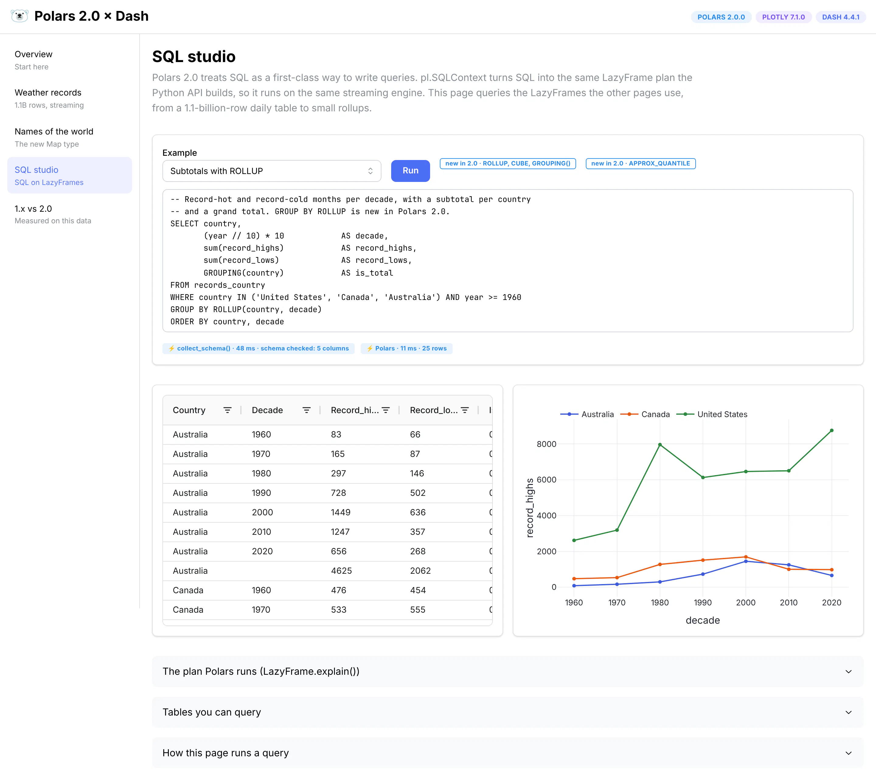
A ROLLUP query over the records table. The schema check took 2 ms and the query 10 ms.

Overview of this app

• Write SQL against the app's tables, from the 1.14-billion-row daily table to the small rollups and Overture's cities
• Examples for the new SQL features, and one with a typo to show the error
• The result in Dash AG Grid, a chart drawn from it automatically, and the plan Polars runs

Polars 2.0 features

The 2.0 announcement calls SQL a first-class citizen. pl.SQLContext turns SQL into the same LazyFrame plan the Python API builds, so it runs on the same streaming engine, and you can keep chaining Python methods onto the result. 2.0 adds a lot of SQL, including GROUP BY ROLLUP, CUBE, GROUPING SETS and GROUPING(), APPROX_QUANTILE, window frames for FIRST_VALUE and LAST_VALUE, and a default value for LAG and LEAD.

ROLLUP is useful for dashboards because it returns subtotals and a grand total in the same result as the detail rows:

SQL errors now show up when you ask for the schema. 2.0 resolves SQL lazily, so ctx.execute(sql) only parses the query. The page calls collect_schema() next, which resolves every table and column in a few milliseconds without reading data, and a typo comes back with a suggestion:

That's handy in any app that accepts a query from a user or an AI agent, because a bad query fails in milliseconds instead of halfway through a scan of a billion rows.

A few nice patterns

• Block SQL that reads files from the server. Polars SQL can read files directly, not only the tables you register. A query like SELECT * FROM read_csv('/etc/passwd') tells Polars to open that file from the server's disk. When we tried it, Polars did open the file and only failed because /etc/passwd isn't a valid CSV. A CSV or Parquet file with something sensitive in it would have come back as rows in the user's browser. So if people can type SQL into your app, register only the tables you want them to see, and refuse any query that calls a file-reading function before you run it. This page does that with a short check:

A check like this is a first line of defense. Also run the app under an account that can't read anything it doesn't need.

• Cap the rows before collecting. The page runs lf.head(5_000).collect(), so a SELECT * over the daily table returns 5,000 rows in milliseconds instead of trying to send a billion rows to the browser.

Polars 1.44 vs 2.0, measured

The biggest performance change in 2.0 comes from the new default: collect() now uses the streaming engine. Polars 1.44 could already stream if you passed engine="streaming", and if your app already does that, you'll see much less of a change. Simple aggregations ran at about the same speed, and the gains were on window functions, sorts and the largest jobs. So we ran 1.44 both ways, and 2.0 with no settings at all.

The tasks are the kind a Dash app or its scheduled jobs run all the time, on the GHCN weather data at two sizes: ten years (2015 to 2024, 119 million rows) and every year (1.14 billion rows). Each run is a new Python process, and the time includes reading the Parquet files from disk. We report the best of up to three runs and the peak memory of the process. The machine was a general-purpose Linux cloud VM (not Plotly Cloud) with 4 vCPUs and 16 GB of RAM, and a watchdog stopped any run that used more than 12 GB, which the table marks as "out of memory".

Best of up to three runs; each run is a fresh process. Python 3.13, Polars 1.44.2 and 2.0.0, 4 vCPU / 16 GB general-purpose Linux cloud VM. The sorts ran with a 14.5 GB watchdog instead of 12 GB, so that 2.0 had room to reach its spill threshold.

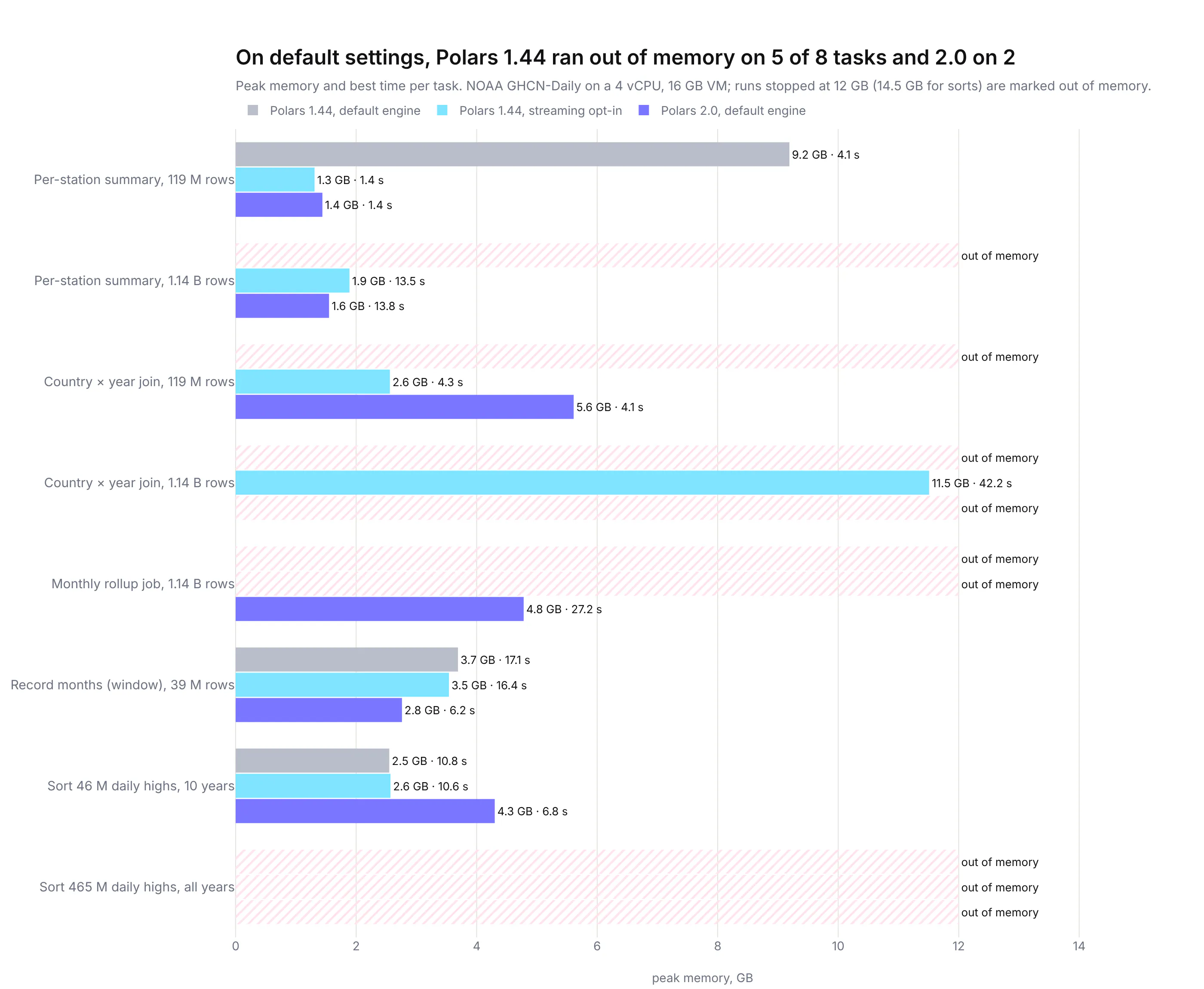
Peak memory and best time per task. Runs that ran out of memory are hatched.

The new default is the big change. On its default engine, Polars 1.44 ran out of memory on five of the eight large tasks, against two for 2.0. One of the five was a per-station summary of 119 million rows that 2.0 finished in 1.4 seconds with 1.4 GB. A Dash app that never mentions an engine gets that improvement just by upgrading.

2.0 also beats 1.44 with streaming turned on. It finished the monthly rollup job over all 1.14 billion rows in 27 seconds with a 4.8 GB peak, where 1.44's streaming engine ran out of memory. The record-finding window function ran 2.7 times faster (6.2 seconds against 16.5). Sorting the 46 million daily highs from ten years took 6.8 seconds against 10.6, though 2.0 used more memory to do it. On simple aggregations the two streaming engines were about the same speed.

Joins are where 2.0 still needs memory. On the country-by-year query, which joins every reading to the stations table, 2.0 used 5.6 GB at ten years where 1.44's streaming engine used 2.6 GB, and on the full table 2.0 ran out of memory while 1.44 finished in 42 seconds using 11.5 GB. The Polars team lists out-of-core joins and group-bys as next on the roadmap. Until then, the easy fix in a Dash app is to join after aggregating: join the stations table to the 39-million-row monthly rollup, or to the result of a group_by, rather than to the raw daily table.

Out-of-core sorting needs disk as well as memory. Sorting all 465 million daily highs crashed every setup on this machine, 2.0 included: the operating system killed each one at about 14 GB. 2.0 starts spilling at about 80% of RAM, which on a 16 GB VM leaves little headroom for everything else. When we lowered the threshold with POLARS_OOC_MEMORY_BUDGET_MB=6000, a setting we found in Polars' source that isn't in the docs yet, memory stayed under 7 GB and Polars spilled to disk as designed. It then stopped with "query aborted, raise POLARS_OOC_DISK_BUDGET_MB" after using the 24 GB of scratch space we allowed, which was about all the free disk the VM had. So plan for scratch disk several times the size of the data you sort.

This benchmark has limits. It's one 4-vCPU machine, one dataset and nine tasks. The Polars team's own benchmarks use TPC-H and TPC-DS on much bigger machines. Test your own queries on the hardware your app runs on. For Polars 2.0 next to DuckDB 2.0 and pandas 3.0 on the same weather data, see our three-way benchmark.

What's new in Polars 2.0

The release post and the upgrade guide have the full list. These are the changes we think matter most if you build Dash apps.

Things that tripped us up

The Polars team wrote a thorough upgrade guide, and most of our changes were in it. These are the ones we hit while building the app:

1. .cast(pl.Date) on a string column now raises "casting from string to date is not supported", where 1.44 parsed the string. Use pl.col("date").str.to_date("%Y%m%d"), which is clearer anyway. NOAA stores dates as "20240101" strings, so this is the first thing a GHCN prep script hits.
2. is_in no longer converts types for you. Checking an integer column against [1.0, 2.5] used to work and now raises InvalidOperationError. Cast one side explicitly.
3. group_by(...).count() is gone. It raises AttributeRemovedError with the message "use GroupBy.len instead", which is about as helpful as an upgrade error can be.
4. cut() and qcut() print a deprecation warning. Their replacements, bin_intervals() and bin_quantiles(), require you to choose labels and are left-closed by default, so check your bin edges if you rely on (a, b] intervals.
5. Map columns can't be read from SQL yet. SELECT names['ja'] FROM cities fails with "expected List data type for list operation, got: Map(String, String)". Use the Python .map.get() expression for now, and chain it onto the SQL result if you need both.
6. Joins no longer keep your row order. We joined 2024's 12 million daily readings to the stations table on both versions. Polars 1.44 returned them in the original order, and 2.0 didn't. A line chart drawn from that result would zigzag. Sort explicitly before drawing lines, or pass maintain_order="left" to join, which gave us the original order back. The same goes for group_by and unpivot.
7. A window over millions of tiny groups is slow. Our first record-finding query, with one window per station and calendar day, took 48 seconds for one year of data. Rolling up to months first fixed it (see the weather records section). Polars 1.44 was slower still on the same query, at 84 seconds.
8. A killed query leaves its spill files behind. After the operating system killed our full-table sort, 11 GB of spill files stayed in /var/tmp/polars-unknown/spill. On a server where jobs share a disk, check for that folder after a crash and clean it up.

How the app talks to Polars

Every page reads data through one small module, data.py. It defines each dataset as a LazyFrame at import time, which costs nothing because a LazyFrame is only a plan:

A callback then adds whatever filter its inputs ask for, collects, and passes the Polars DataFrame to Plotly Express as it is:

Nothing is loaded when the app starts, so it starts quickly and each gunicorn worker only holds what its current callbacks are using. Compare that with df = pd.read_parquet(...) at the top of app.py, where every worker loads its own full copy at startup and keeps it. Polars releases Python's GIL while it works, so several callbacks in the same worker can run queries at once on different threads.

The data.py file also checks where it's running, so the same code works locally, on Plotly Cloud and on Dash Enterprise:

On Plotly Cloud, attach a persistent filesystem at /data and set DATA_DIR=/data. On Dash Enterprise, turn on the app's persistent filesystem and the code finds it at ../mount. The rollup job writes every file under a temporary name and renames it into place, so it's safe to run on a schedule while the app is serving. Our DuckDB 2.0 post has more on persistent filesystems and on replacing per-click warehouse queries with this pattern.

Bonus: the app is also a tool for AI agents

The app is created with Dash(__name__, enable_mcp=True), which turns on Dash MCP. That exposes the app's callbacks as tools that AI agents like Claude Code, Cursor or ChatGPT can call. Ask an agent connected to the app "how many record-hot months did Australia set since 2015?" and it calls the same callback your users trigger from the country dropdown, backed by the same Polars query. The SQL studio's collect_schema() check is useful here too, because an agent that writes a bad query gets a precise error back in milliseconds and can fix it.

Thank you, Polars team

We've been big fans of Polars for a long time, and 2.0 is a big step for anyone running Polars in Dash. The streaming engine is now the default, out-of-core sorting works on an ordinary machine, and the release removed years of legacy API with error messages that tell you exactly what to write instead. 41 people are credited on the 2.0.0 release notes alone, on top of everyone who built the streaming engine over the past few releases.

Thank you to Ritchie Vink and everyone at Polars and in the community who made this release. Plotly users have been able to use Polars for a while, because since plotly.py 6.0 Plotly Express has read Polars DataFrames natively through Narwhals, with no copy to pandas. If you build something with Polars and Dash, we'd love to see it.

Getting started with Polars 2.0 in Dash

If you already use Polars in a Dash app, upgrade, run the app and read the errors: most removed APIs fail with the name of their replacement. Then look for join and group_by results that feed line charts or tables without a sort.

If your app uses pandas, find the slowest callback and rewrite just that one with pl.scan_parquet(...), a filter and collect(). Plotly Express takes the Polars result directly, so nothing else in the callback has to change.

When you're ready to deploy, publish to Plotly Cloud with a persistent filesystem mounted at /data, or deploy to Dash Enterprise with the persistent filesystem turned on. If you're a Dash Enterprise customer and want help moving big dashboards onto this pattern, talk to your Plotly team.

Every Polars 2.0 feature in this post