Gauge Charts - A Complete Guide

TL;DR

• A gauge chart shows one value on a curved scale against a target, a limit or a set of bands. In Plotly it's go.Indicator with mode="gauge+number+delta".
• Gauge charts are also known as speedometer charts, dial charts and radial gauges, and are similar to bullet charts.
• Use one when a single KPI against a known target or official bands is the whole message: storage against its seasonal average, debt against its legal limit, air quality against EPA's categories.
• Gauges take a lot of space for one number and show no history, so use a bullet gauge for a panel of KPIs, a number with a sparkline when the trend matters, and a line chart for anything over time.
• Any coding agent can make one with Plotly in a minute, and make_subplots(specs=[[{"type": "indicator"}]]) puts several in one dashboard figure.

What is a gauge chart?

Gauge charts look like this:

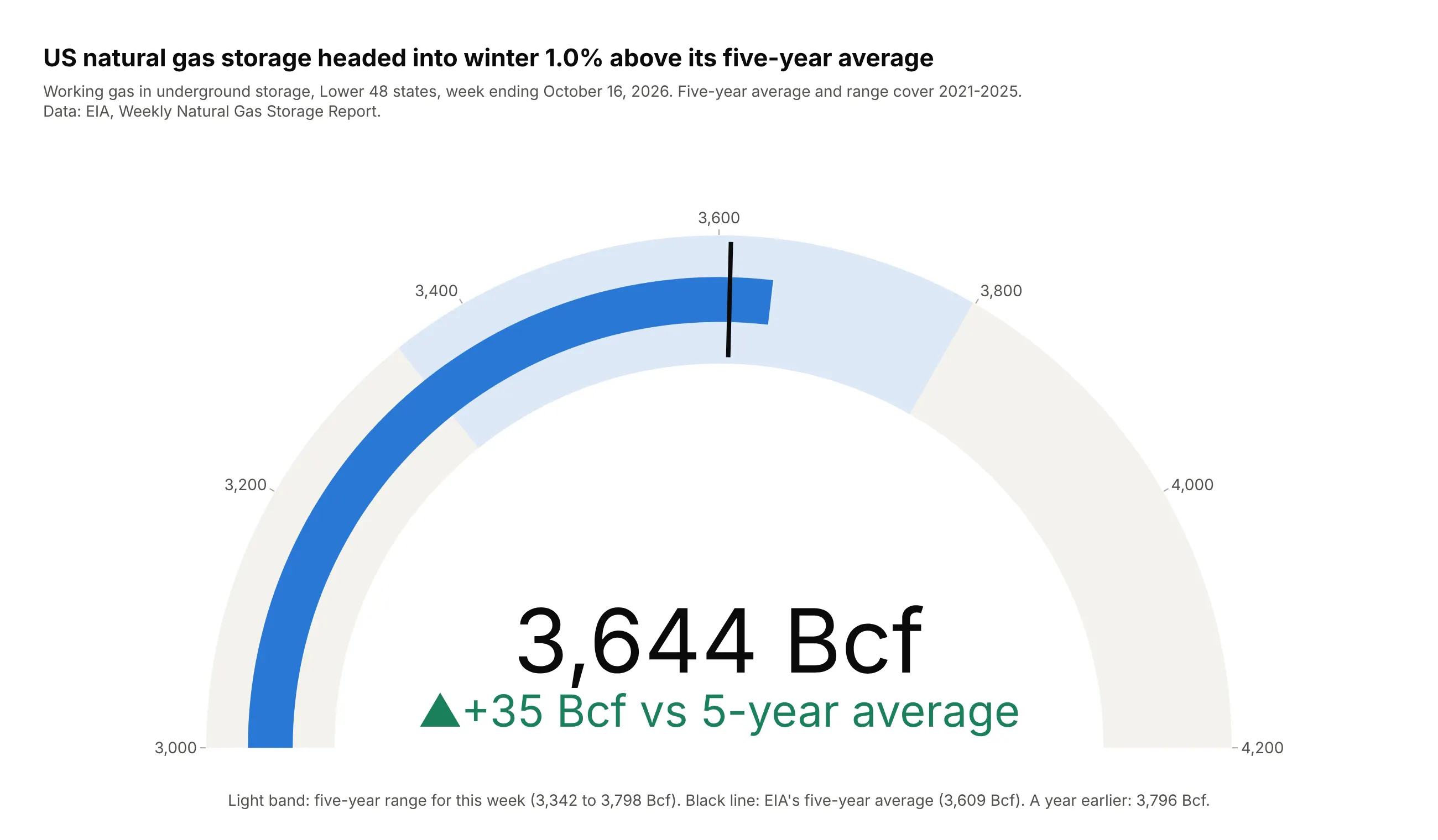
Data: EIA, Weekly Natural Gas Storage Report, week ending October 16, 2026.

How do you read a gauge chart? In the example above, notice these things:

• The blue bar is the value, the natural gas held in US storage in mid-October, and it fills the dial clockwise from the left end. The big number in the middle gives the same value, 3,644 billion cubic feet, so nobody has to read it off the arc.
• The black line is the target the value is compared with, EIA's five-year average for the same week. The blue bar ends just past the line, which means storage is a little above normal.
• The light blue band is the five-year range for this week, so a bar that ends inside it is within what the past five years have seen for mid-October.
• The green number under the dial states the gap to the average, +35 Bcf, and the up arrow and the color say which way it goes.
• The dial starts at 3,000 Bcf instead of zero, which makes a small gap easy to see. The length of the bar is therefore not a share of anything, and a bar that fills half the arc does not mean storage is half full.

It's often used for charts like these:

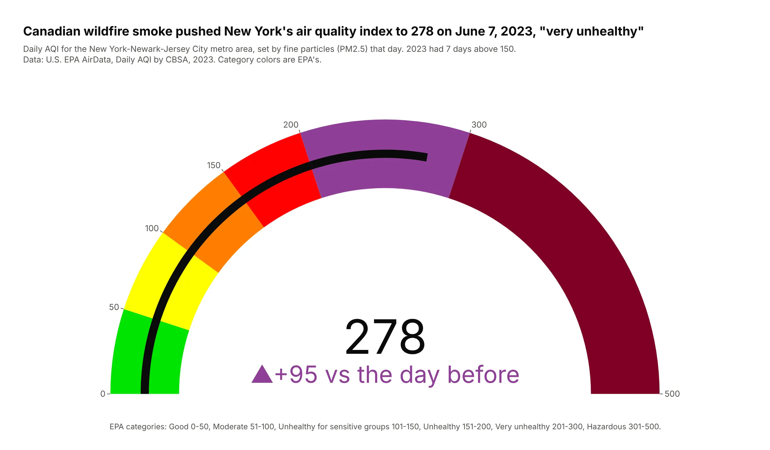
A reading on a scale with official bands. Canadian wildfire smoke pushed New York's daily air quality index to 278 on June 7, 2023, inside EPA's purple "very unhealthy" band. Data: U.S. EPA AirData, Daily AQI by CBSA.

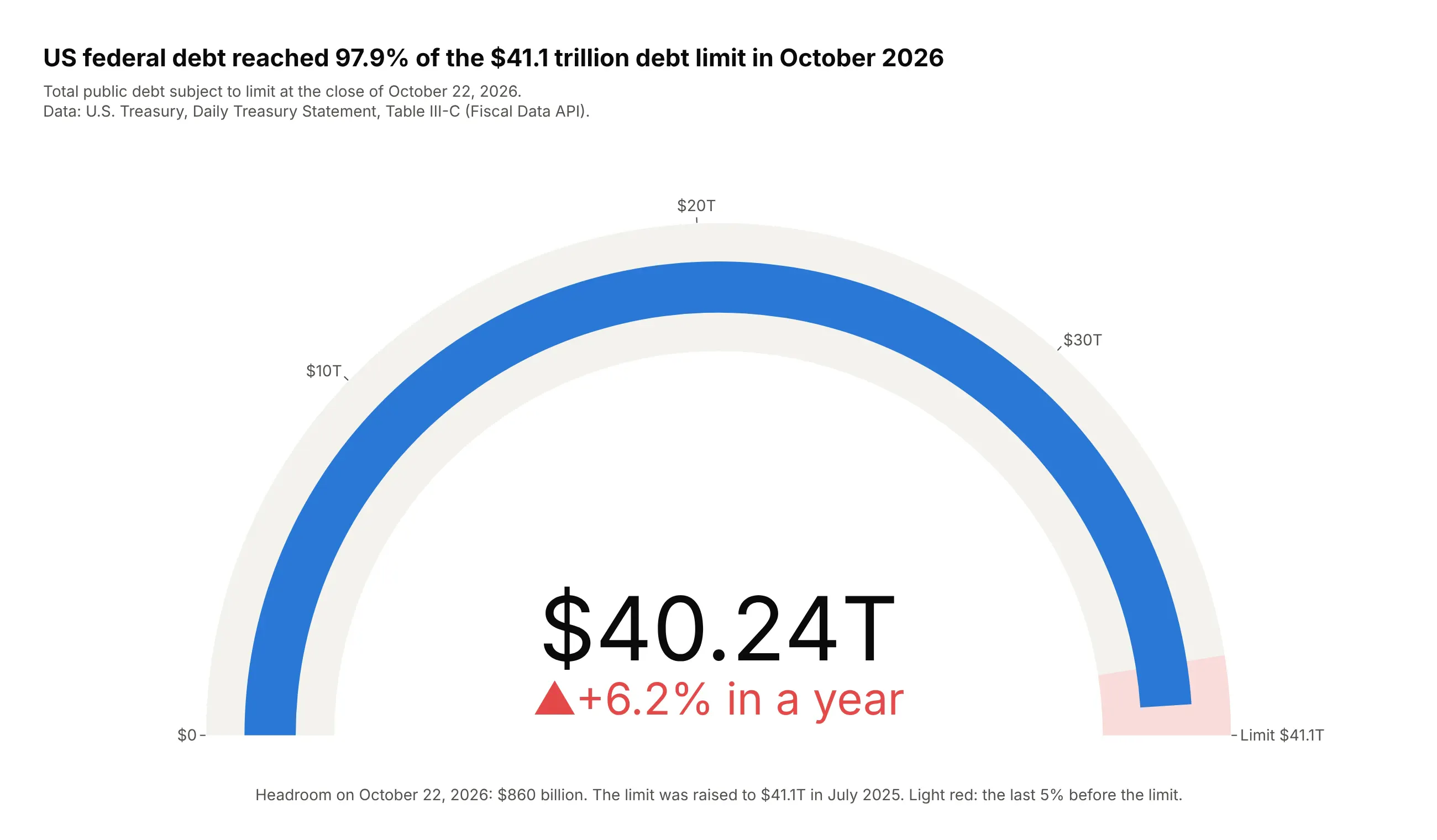
A stock growing toward a hard limit. US federal debt subject to the limit reached $40.24 trillion on October 22, 2026, 97.9% of the $41.1 trillion ceiling, so the empty sliver of the arc is the $860 billion of headroom. Data: U.S. Treasury, Daily Treasury Statement, Table III-C.

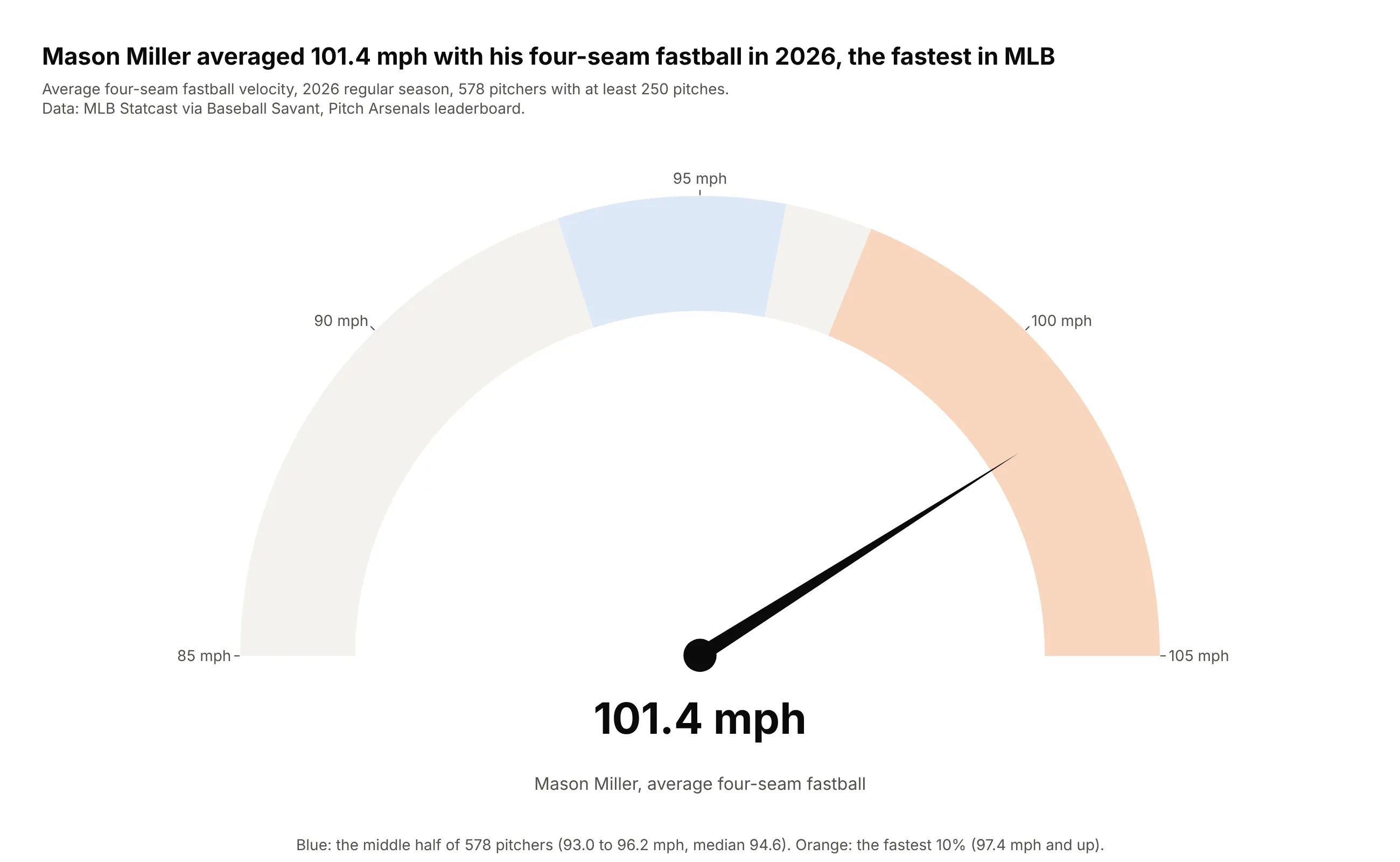
A speed, where the speedometer is literal. Mason Miller's four-seam fastball averaged 101.4 mph in 2026, the fastest of 578 pitchers; the median was 94.6 mph. Data: MLB Statcast via Baseball Savant.

A short history

Dials came to dashboards from cars and control rooms, and in Information Dashboard Design (2006) Stephen Few argued they waste space and are hard to compare. He designed the bullet graph to replace them; his Bullet Graph Design Specification puts the same measure, target and bands on a straight line, because people judge position along a common scale more accurately than angle (Cleveland and McGill, 1984). Plotly's go.Indicator draws both, with gauge.shape="angular" or "bullet".

Alternatives to a gauge chart

Here's the same inflation reading drawn six ways. Some are better for the question, some worse, some just different:

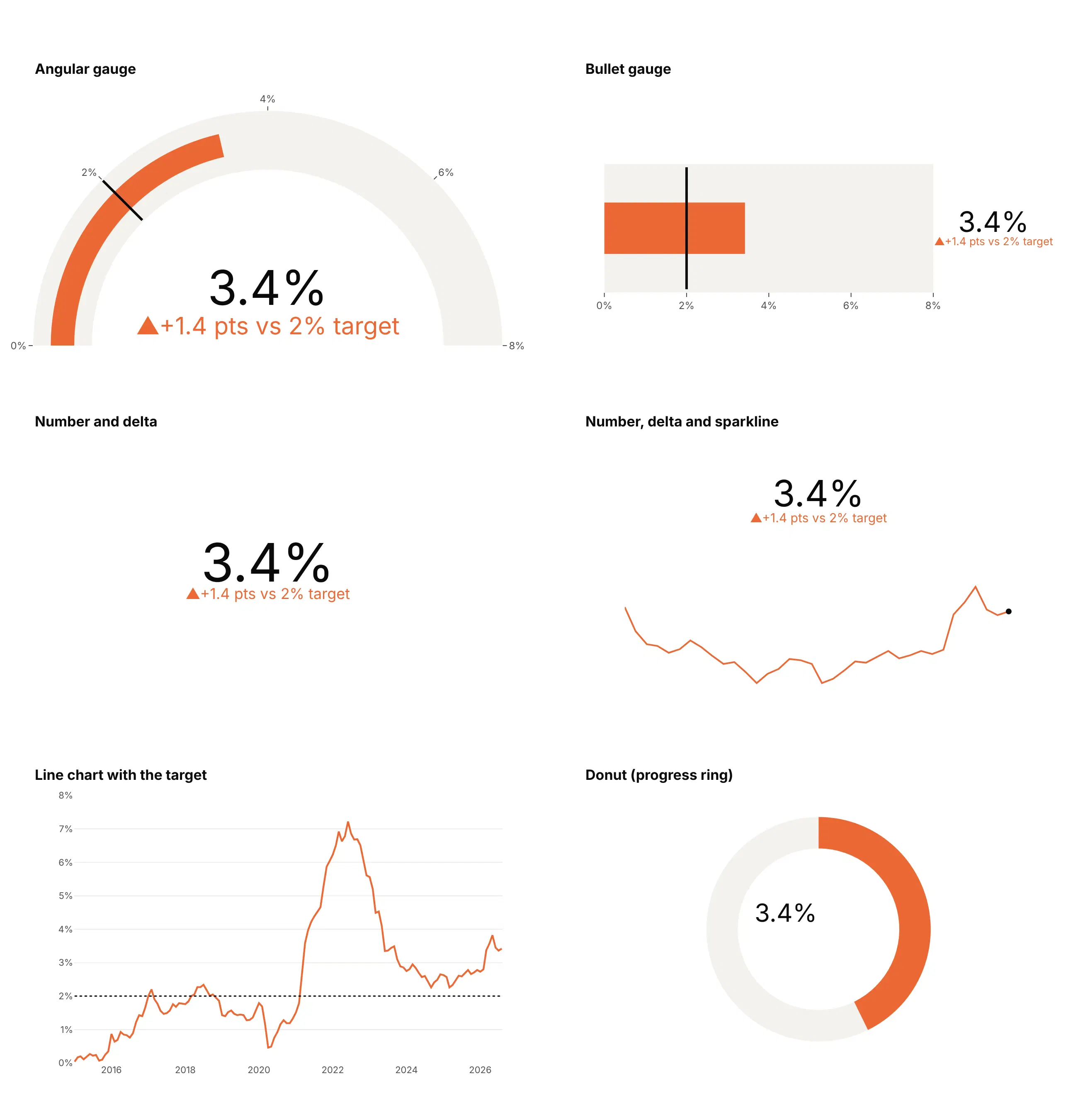
• Bullet gauge (better for a panel of KPIs). The same value, target and bands in a strip, so several stack into one panel on a shared scale and are read more accurately than angles.
• Number and delta (better when space is tight). A big number and its gap to the target say the same thing in a tenth of the space; it's the standard KPI card.
• Number, delta and sparkline (better when the trend matters). Adds the last three years, which shows that inflation rose again in 2026, something no gauge can show.
• Line chart with the target (better for history). Shows that PCE inflation has been above 2% since March 2021. Use it whenever the question is "how did we get here".
• Angular gauge (works too, for one KPI on a big screen). Familiar and readable from across a room, but it takes the most space.
• Donut or progress ring (worse). A ring reads as a share of a whole, and here the 8% maximum is arbitrary, so "3.4 out of 8" means nothing.

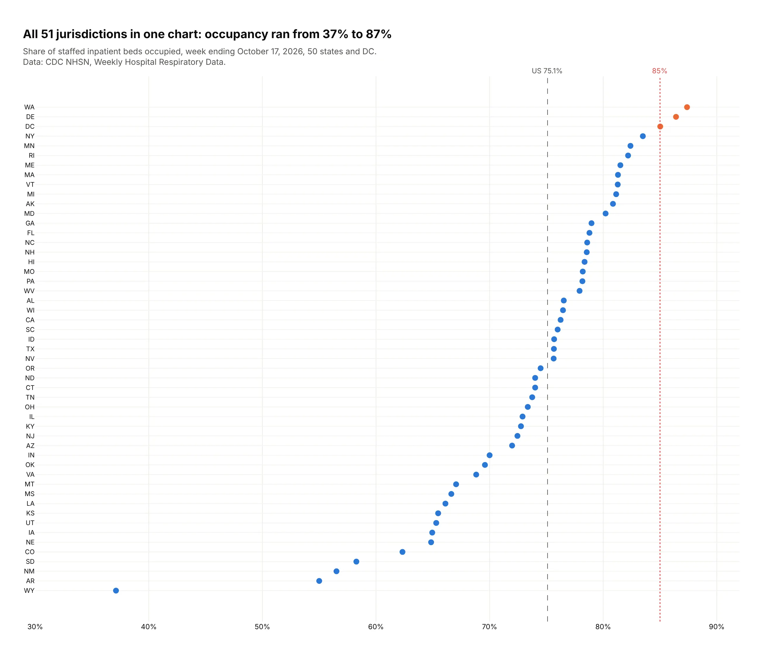
Here's where a dot plot wins. Twelve gauges fill a screen, while one dot plot shows the bed occupancy of all 50 states and DC against the same 85% line:

How to make a gauge chart

With AI

ChatGPT, Claude Code, GitHub Copilot, Cursor and other AI tools are excellent at writing Plotly code. Name Plotly in the prompt, and say what the range, the target and the bands are:

With Plotly Studio

Plotly Studio is a desktop app where you point an AI at a dataset and it builds charts and a Dash app around your questions. Ask for a gauge the same way:

Show the latest weekly gas storage as a gauge from 3,000 to 4,200 Bcf, with the five-year range for the same week as a light band and the five-year average as a black threshold line. Show the difference from the average under the number, and add a line chart below of this year against the five-year range.

Make a gauge chart in Python or JavaScript

This is the code AI tools write under the hood. In Python:

In JavaScript, plotly.js takes the same attributes. This draws a circular gauge, the default gauge.shape: "angular", and gauge.shape: "bullet" turns it into a linear gauge on a straight scale:

Plotly colors a rising delta green by default, so set delta.increasing.color to red whenever up is bad, as it is for inflation.

Share it

Every Plotly chart has a Share chart button (the cloud icon in its toolbar) that uploads it to Plotly Cloud and gives you a link. Only you can see it until you change its visibility.

For a live app, put the chart in a Dash app and publish it with the Plotly Cloud CLI. Coding agents can run these commands for you:

If your data has to stay in your own cloud or data center, publish to Dash Enterprise instead.

Dos and don'ts

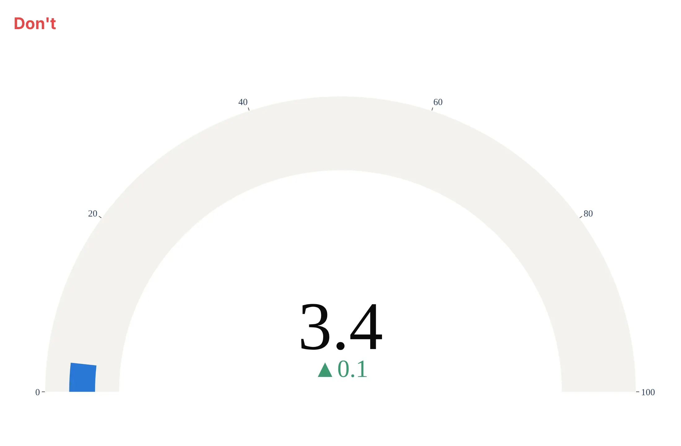
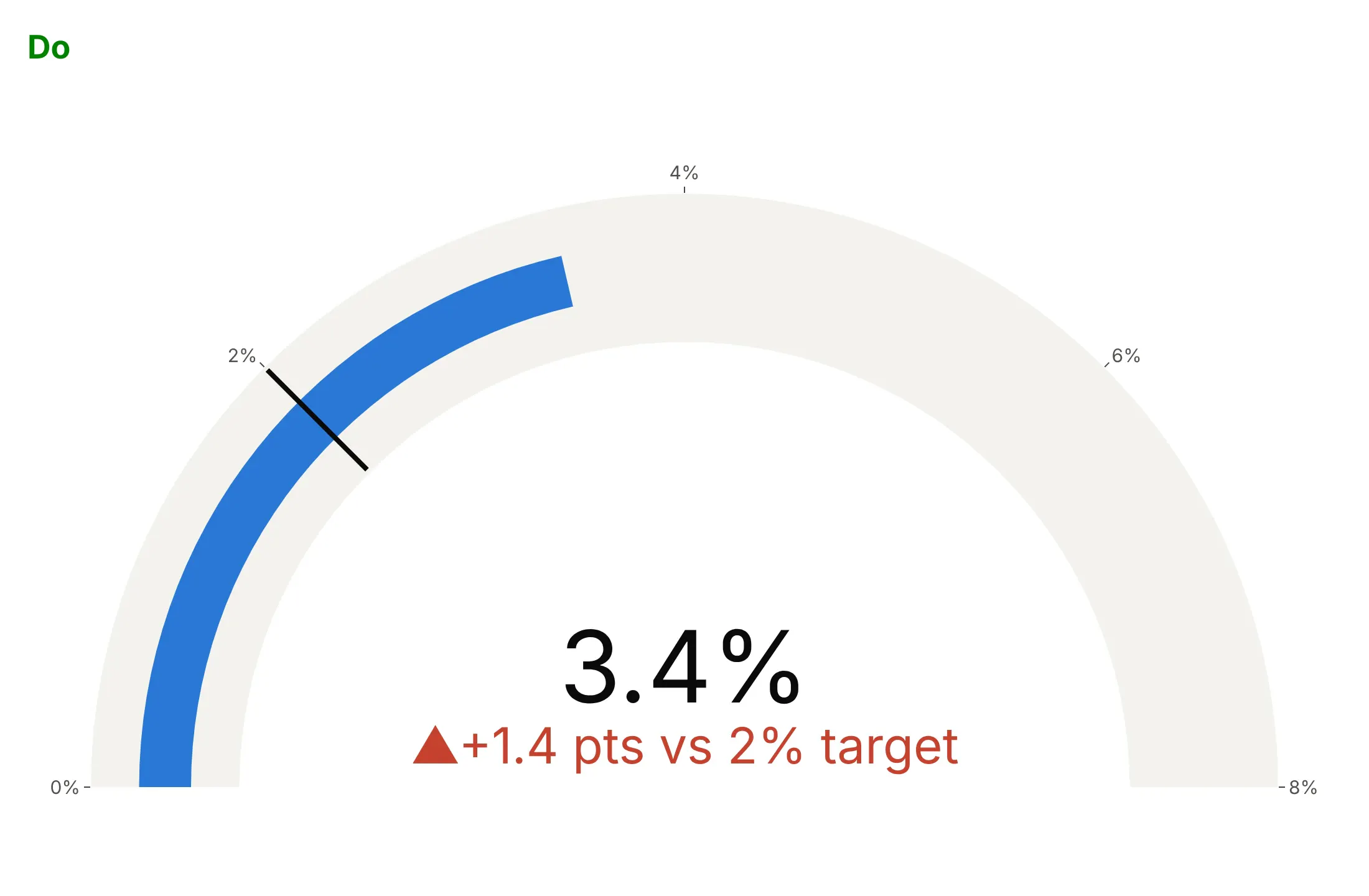
A gauge is only as good as its range and its reference. Here is the same August 2026 inflation reading both ways, in the same colors.

Don't use a 0-100 axis for a 3.4% rate, leave out the target and the units, compare with last month and let a rise in inflation show in green, or switch to a serif font:

Do fit the axis to the data (0-8%), draw the 2% target as a threshold, measure the delta from the target and color it red because higher inflation is bad:

Checklist

Do

• Write a title that states the takeaway with the number, like "PCE inflation was 3.4% in August 2026, 1.4 points above the Fed's 2% target."
• Set gauge.axis.range on purpose: above zero when the action is in a narrow band, ending at a real maximum when there is one.
• Show the target as a threshold and reference the delta to it when distance from target is the question.
• Use steps only for bands that mean something: a normal range, official categories, the spread of peers.
• Color deltas by meaning per KPI with delta.increasing.color and delta.decreasing.color.

Don't

• Use traffic-light steps without defined thresholds behind them.
• Fill a screen with gauges when bullets or a dot plot would hold the same values.
• Set the number's font size when a delta sits under it; Plotly sizes both to fit, and a fixed size can push them into each other.
• Rely on color alone for a category; name it in the title.

Options to customize

These are the go.Indicator options that matter most. The full list is in the Plotly indicator documentation and on the gauge charts page.

1. mode: any of number, delta and gauge, joined with +.
2. value: the number shown.
3. number.prefix, number.suffix, number.valueformat: units and a d3 format such as .1f or ,.0f.
4. delta.reference: what the delta compares with, such as a target, last year or an average.
5. delta.relative: show a percent change instead of a difference.
6. delta.increasing.color, delta.decreasing.color, delta.symbol: delta colors and arrows; set them by what's good for each KPI.
7. delta.position: the delta above, below, left or right of the number.
8. gauge.shape: angular (the dial) or bullet (a strip).
9. gauge.axis.range, tickvals, ticktext: the scale and its labels; put units in ticktext.
10. gauge.bar.color, gauge.bar.thickness: the value bar; thickness 0 hides it, for a custom needle.
11. gauge.steps: background bands as {range, color}.
12. gauge.threshold.value, line, thickness: a line at a target or limit.
13. gauge.bgcolor, gauge.borderwidth: the track color and border.
14. title.text, title.align: a short label inside the indicator.
15. domain: where the indicator sits, for several in one figure.
16. make_subplots(specs=[[{"type": "indicator"}]]): indicator cells in a grid, mixed with xy cells for sparklines.

More gauge chart examples

Ten more gauges, bullet gauges and KPI indicators built from real public data, each with its source, the technique that makes it work and a prompt to rebuild it.

1. Lake Mead and the Colorado River shortage tiers

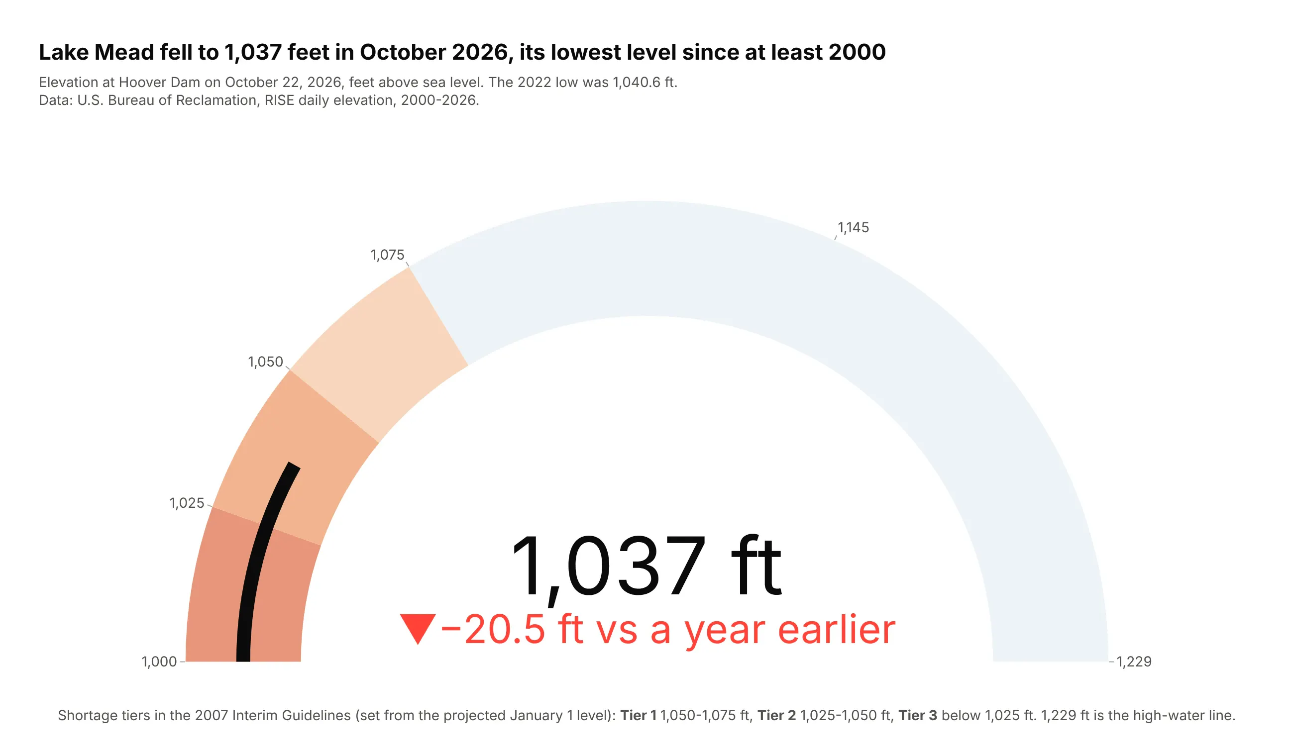
Lake Mead fell to 1,037.2 feet on October 22, 2026, 20.5 feet lower than a year earlier and below its July 2022 low of 1,040.6 feet. That puts it in the 1,025-1,050 foot band of the 2007 Interim Guidelines' second shortage tier.

Data: U.S. Bureau of Reclamation, RISE daily elevation; tiers from the 2007 Record of Decision.

Tip: the steps are the official tiers, darkening as shortages deepen, and tick labels sit on the tier boundaries.

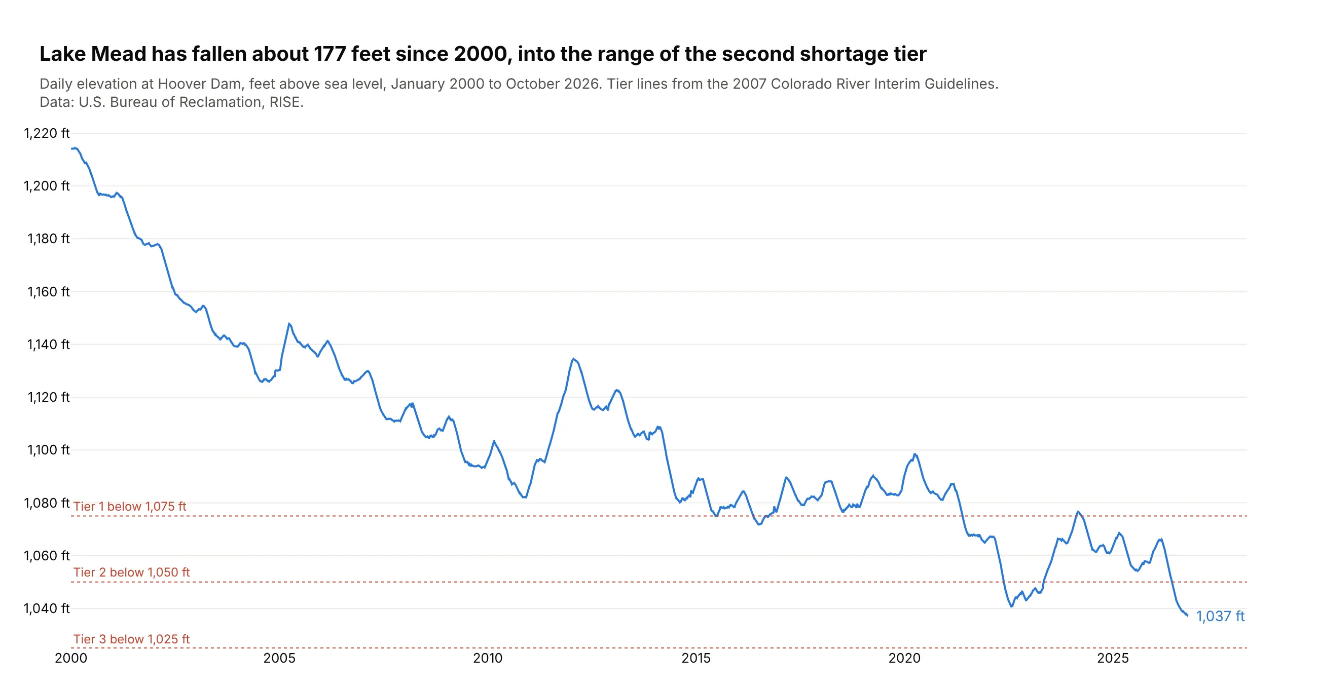
Another way to see it: the daily record since 2000 shows a fall of about 177 feet, with short recoveries.

2. California's largest reservoirs

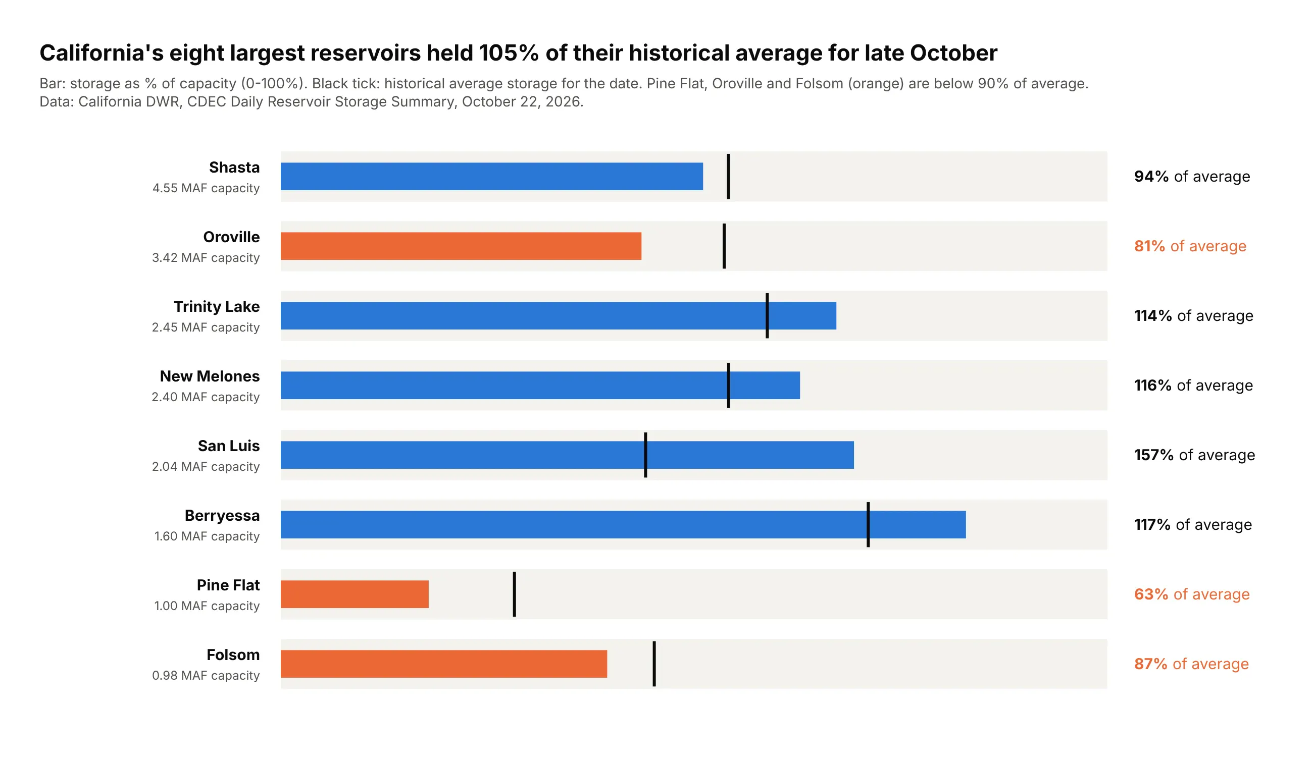
The eight largest reservoirs held 105% of their historical average for October 22, 2026, but not evenly: San Luis was at 157% of average while Pine Flat was at 63% and Oroville at 81%.

Data: California DWR, CDEC Daily Reservoir Storage Summary.

Tip: eight shape="bullet" indicators stacked with domain share one 0-100% scale, which eight angular gauges couldn't.

3. Earth's temperature and the 1.5°C line

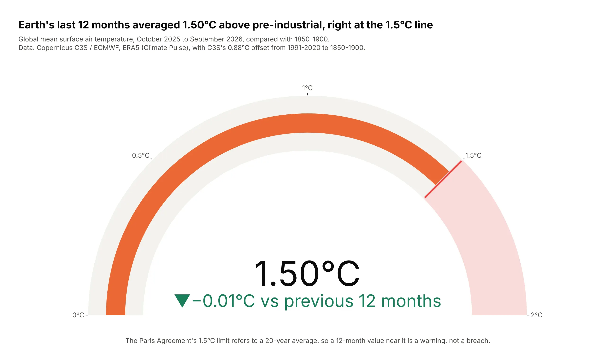
From October 2025 to September 2026, global surface air temperature averaged 1.50°C above 1850-1900 (1.495 before rounding), 0.01°C below the previous 12 months. The calendar year 2024 was 1.60°C.

Data: Copernicus C3S / ECMWF, ERA5 via Climate Pulse, with C3S's 0.88°C offset to pre-industrial (Global Climate Highlights 2024).

Tip: a 12-month average weighted by days steadies the needle, and the note says the Paris limit is a 20-year average.

4. PCE inflation against the Fed's target

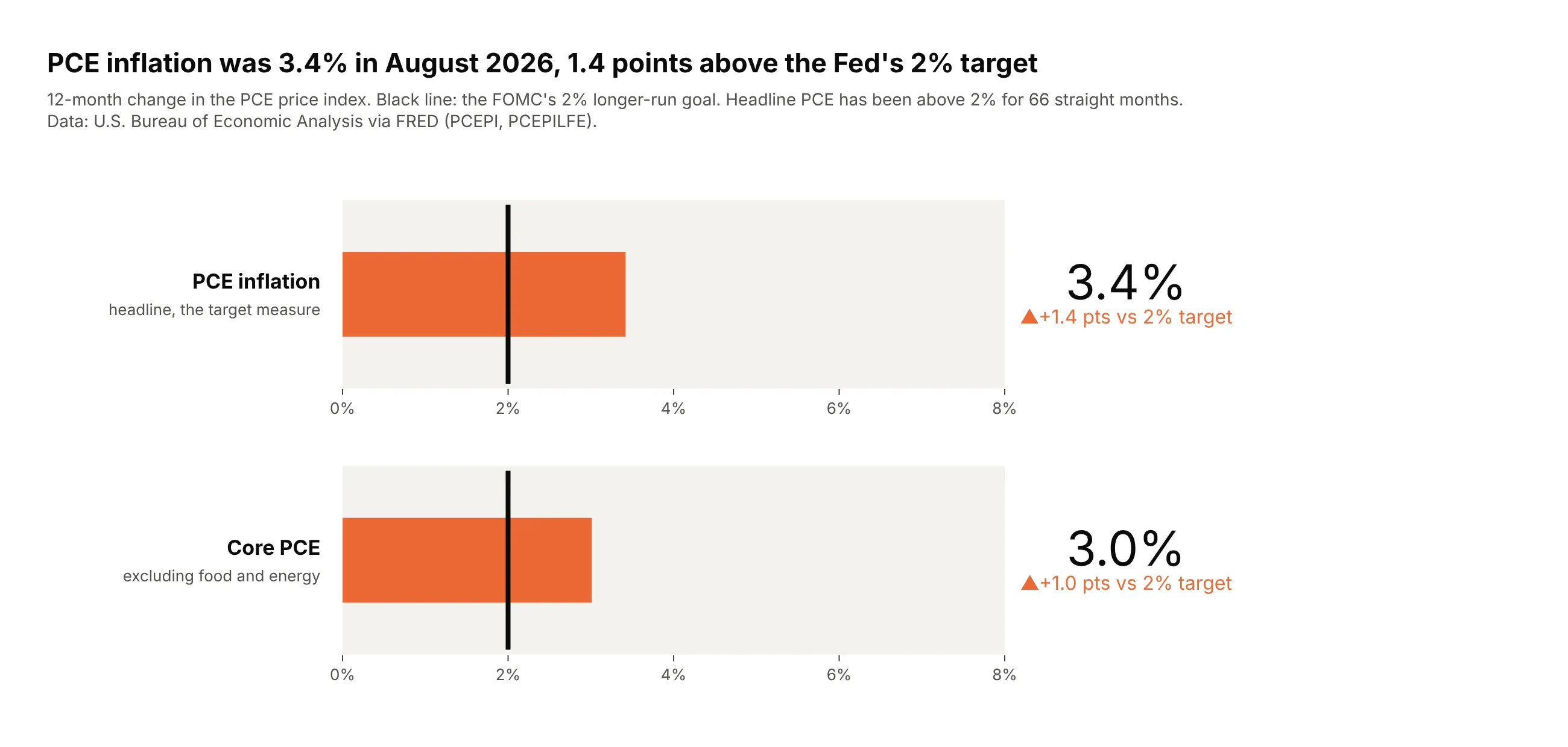
PCE inflation was 3.4% in August 2026 and core PCE 3.0%, 1.4 and 1.0 points above the FOMC's 2% goal. Headline PCE has been above 2% for 66 straight months.

Data: BEA via FRED (PCEPI, PCEPILFE).

Tip: two bullets on one shared axis compare headline and core, and the delta reference is the target.

5. Unemployment against CBO's natural rate

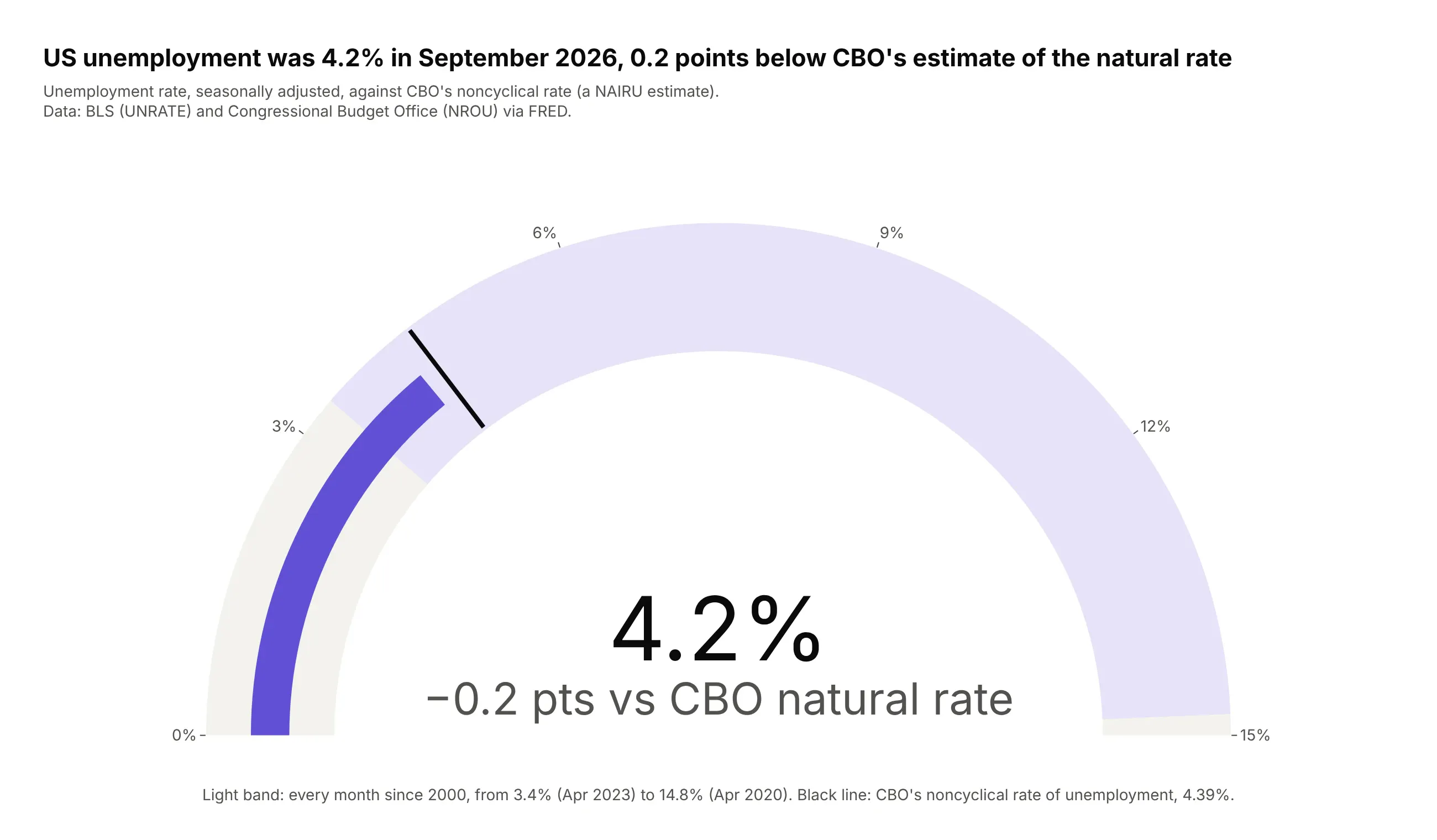
Unemployment was 4.2% in September 2026, 0.2 points below CBO's noncyclical rate of 4.39%. Since 2000 it has ranged from 3.4% to 14.8%.

Data: BLS (UNRATE) and CBO (NROU) via FRED.

Tip: the delta's colors are both gray, because being below or above an estimated natural rate isn't good or bad in itself.

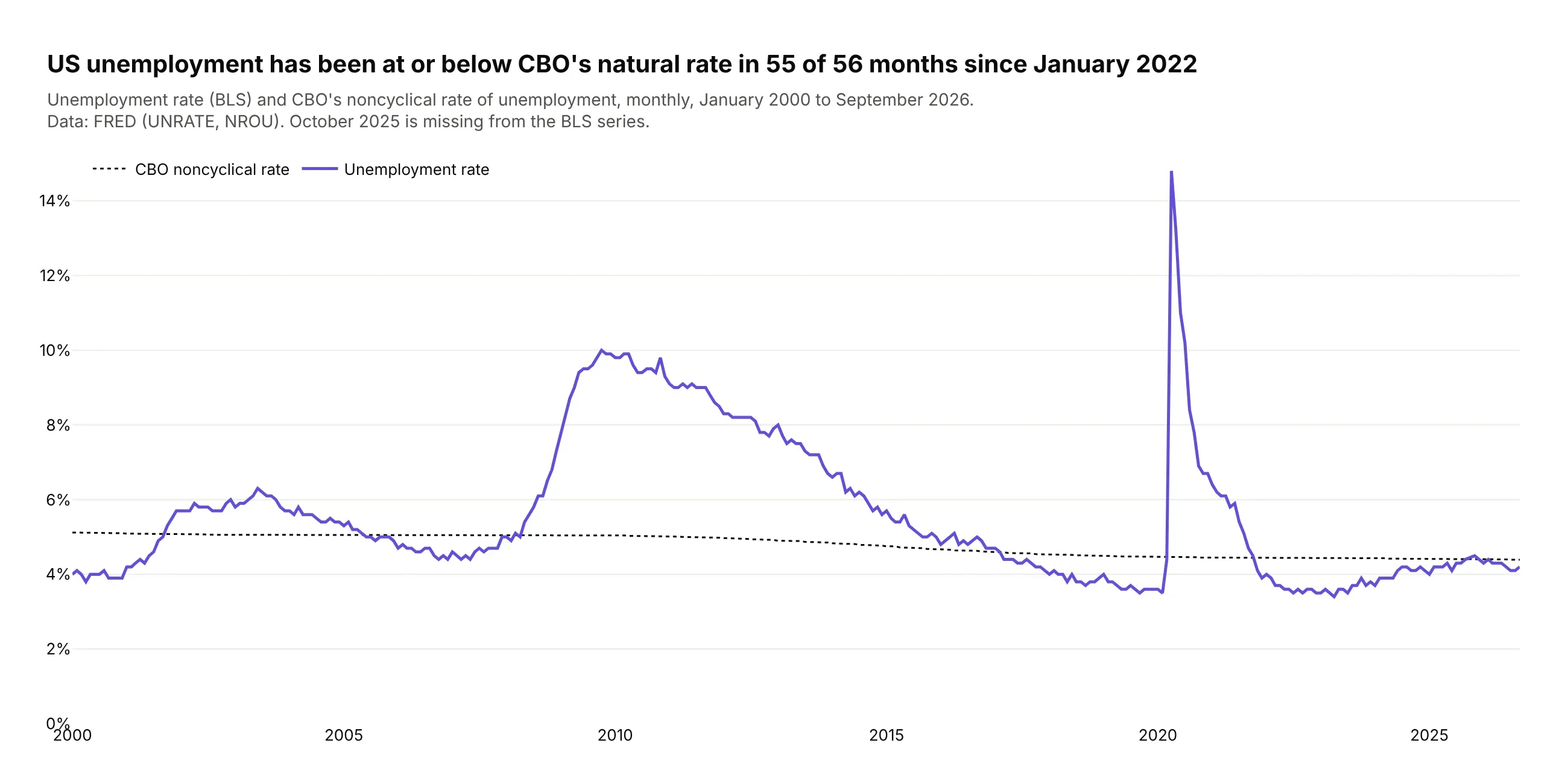
Another way to see it: over time, unemployment has been at or below CBO's estimate in 55 of the 56 months since January 2022.

6. Markets in their 52-week ranges

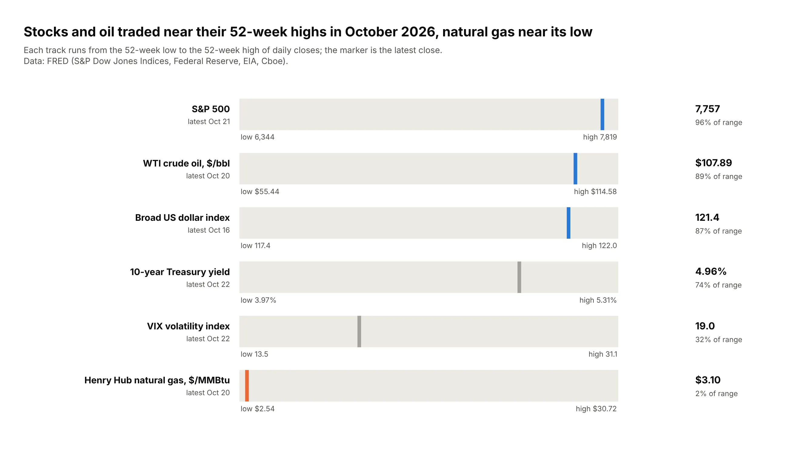
In October 2026 the S&P 500 sat at 96% of its 52-week range and WTI crude at 89%, while Henry Hub gas, at $3.10, was at 2% of a range stretched by a $30.72 spike in January 2026.

Data: FRED (S&P Dow Jones Indices, Federal Reserve, EIA, Cboe).

Tip: rescaling each price to 0-100% of its own range puts an index, a yield and a commodity on one axis; the bar is hidden and the threshold is the marker.

7. A US economy dashboard

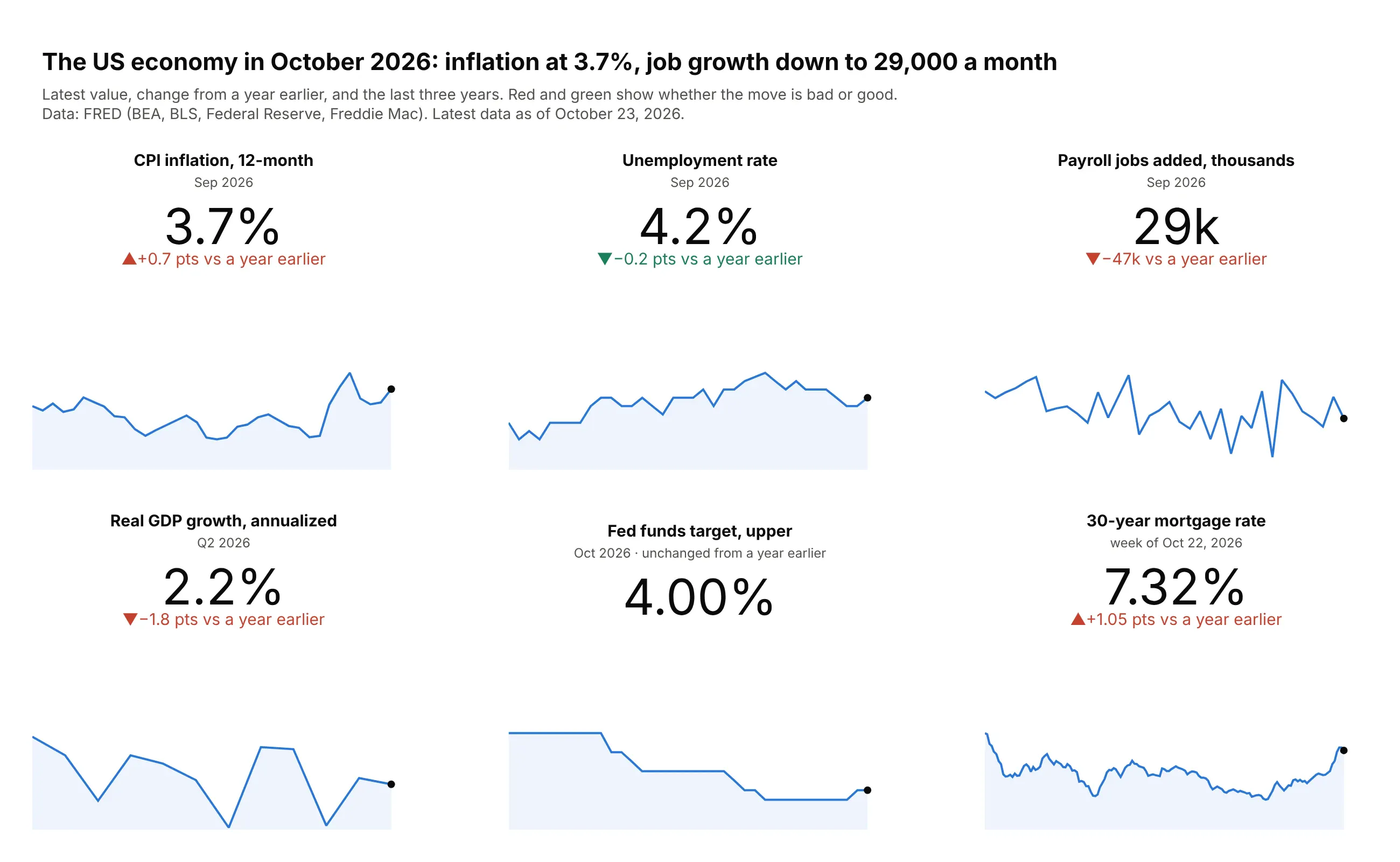
CPI inflation rose to 3.7% in September 2026, 0.7 points higher than a year earlier, while payrolls added 29,000 jobs and the 30-year mortgage rate reached 7.32%.

Data: FRED (BEA, BLS, Federal Reserve, Freddie Mac).

Tip: make_subplots with indicator rows above xy rows puts each number, delta and sparkline in one grid.

8. Hospital bed occupancy by state

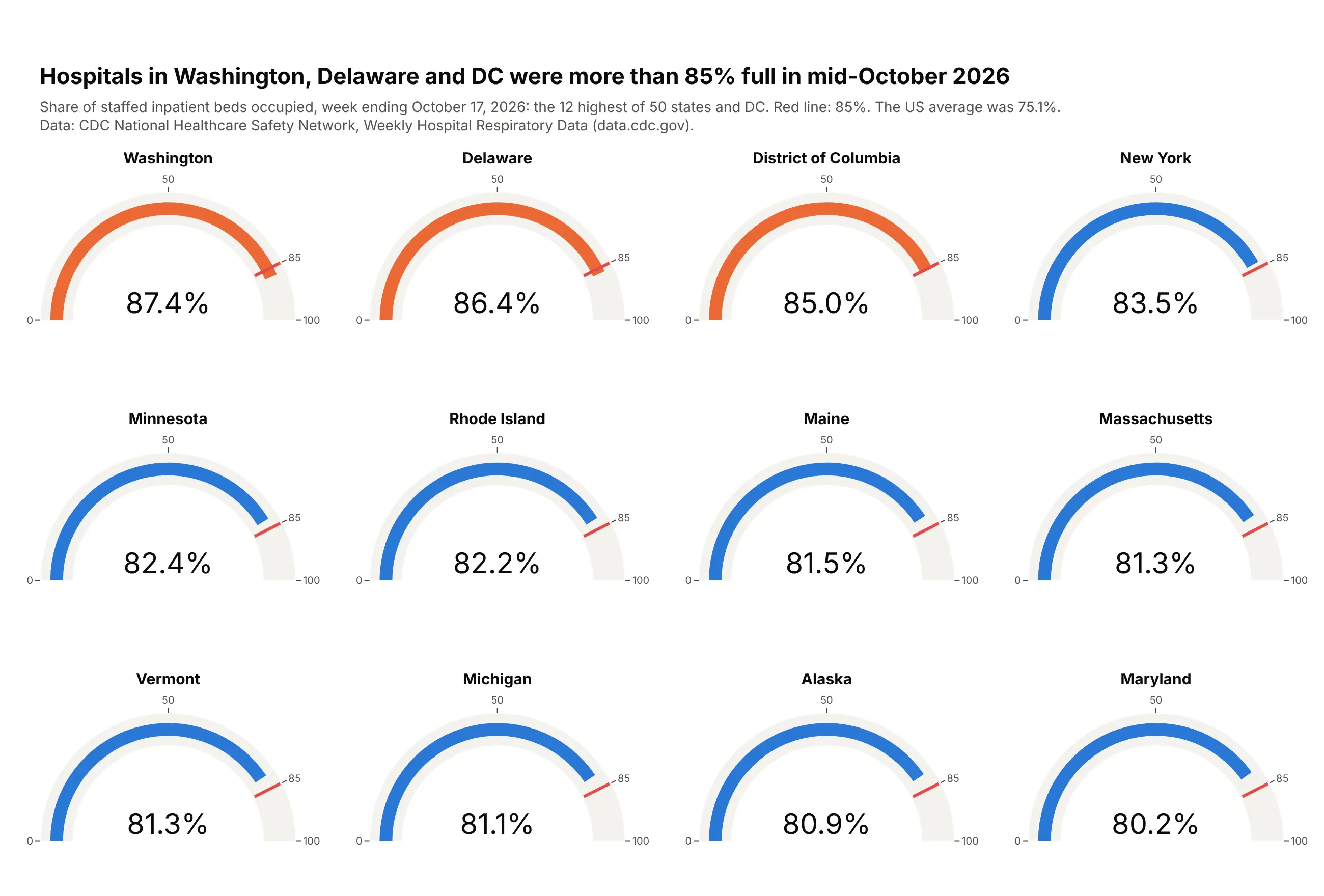
Hospitals in Washington (87.4%), Delaware (86.4%) and DC (85.0%) were above 85% occupancy in the week ending October 17, 2026, a warning level that traces to Bagust et al., 1999. The US average was 75.1%.

Data: CDC NHSN, Weekly Hospital Respiratory Data.

Tip: make_subplots(specs=[[{"type": "indicator"}] * 4] * 3) gives every gauge the same scale and threshold, and only the ones past it turn orange.

9. Kindergarten MMR coverage against the 95% target

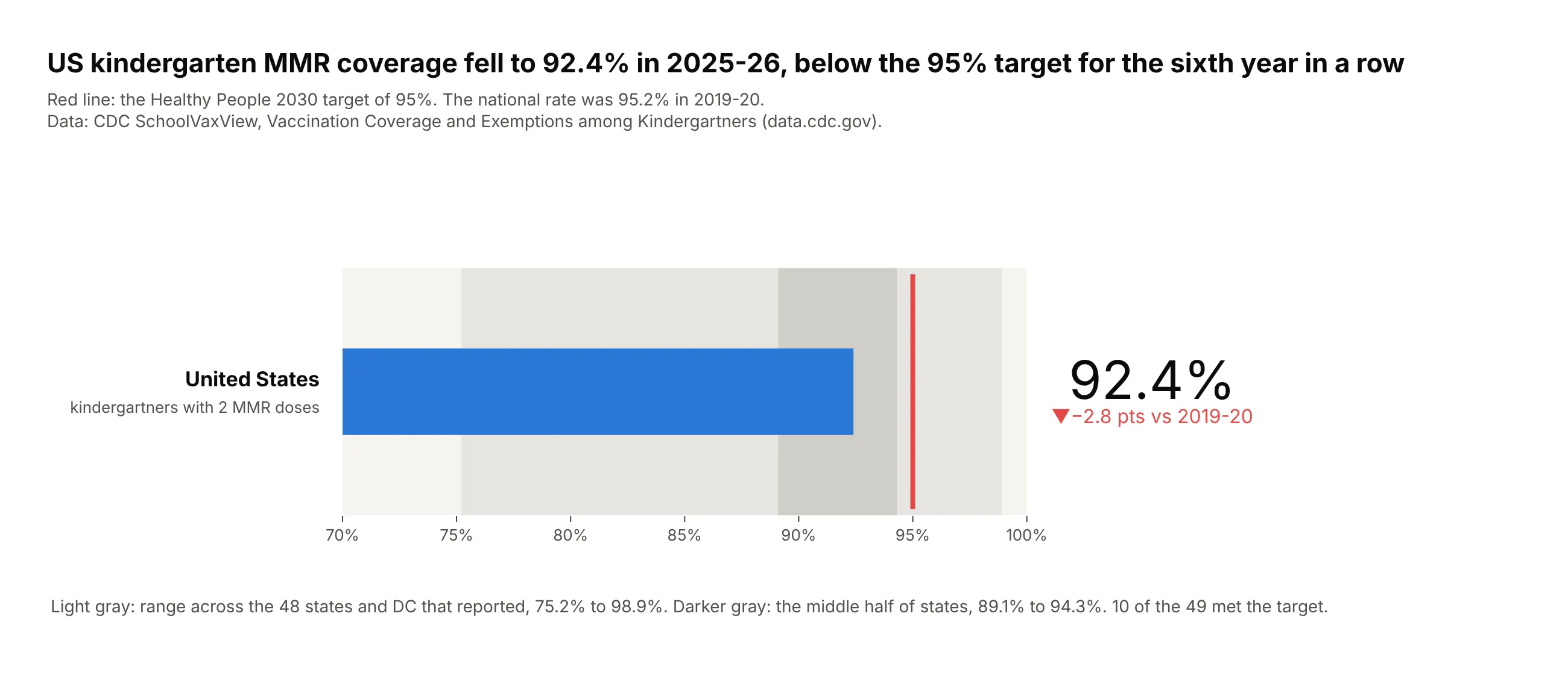
Coverage was 92.4% in 2025-26, 2.8 points below 2019-20 and under the Healthy People 2030 target of 95% for the sixth year in a row. Only 10 of the 49 reporting jurisdictions met it.

Data: CDC SchoolVaxView (data.cdc.gov).

Tip: two steps show the spread of states (full range and middle half) behind the national bar.

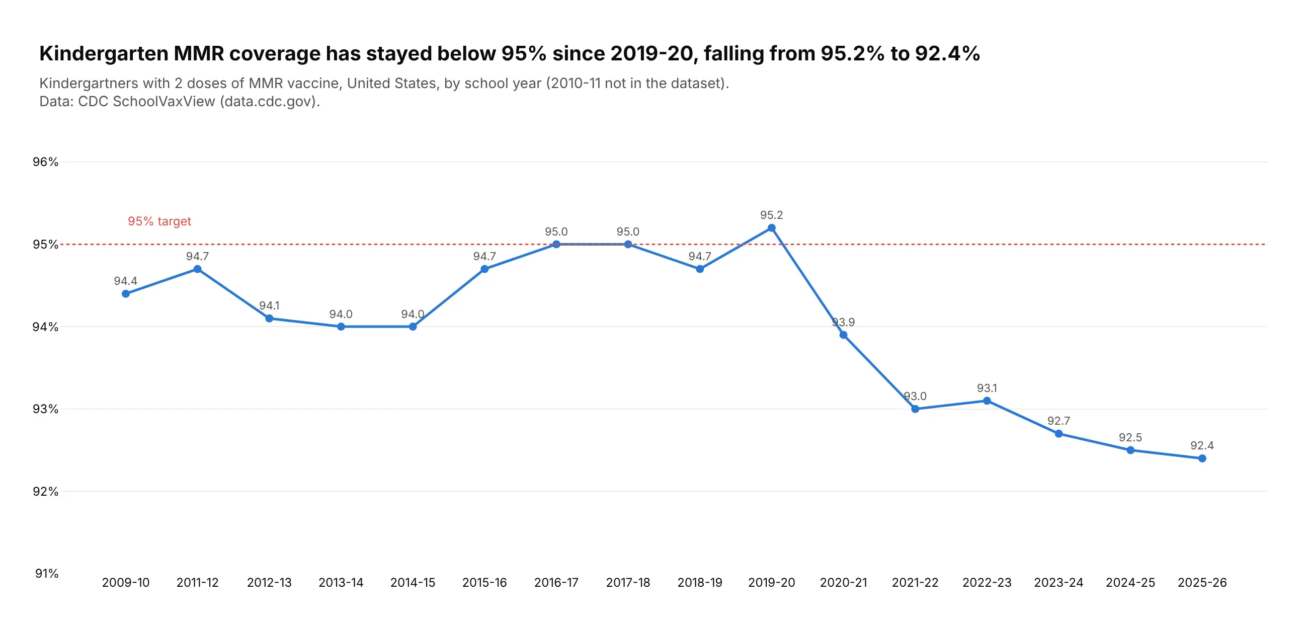
Another way to see it: the national series shows the drop after 2019-20.

10. Medicare Part D's costliest drugs

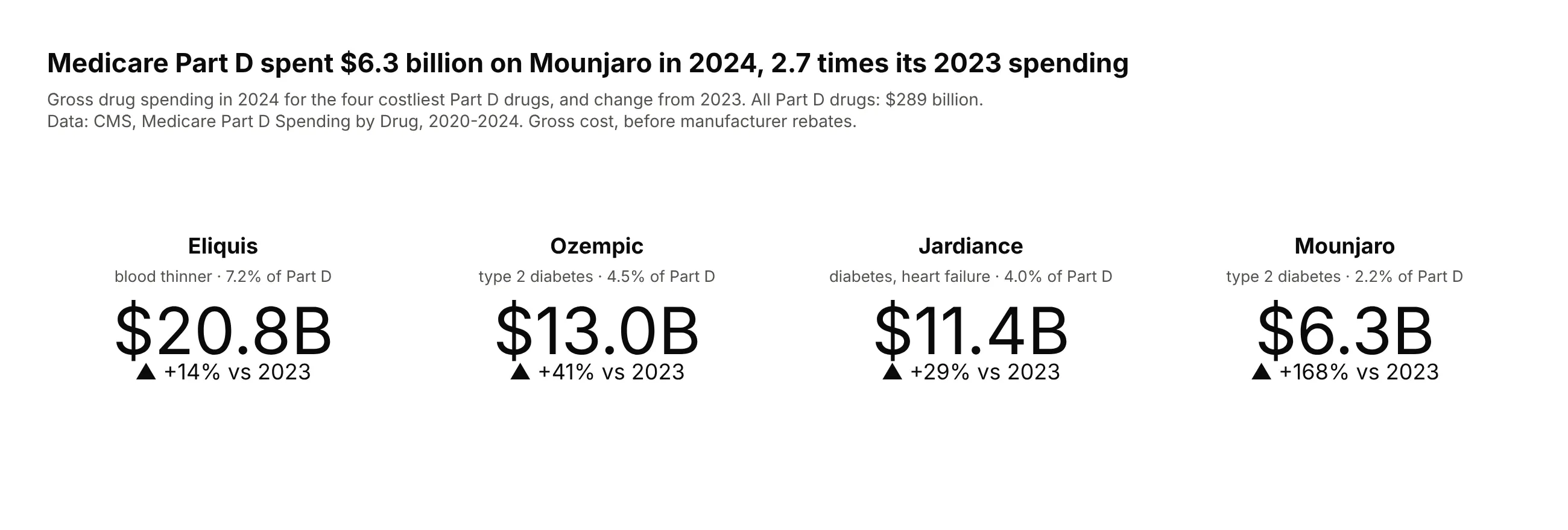
Medicare Part D spent $6.3 billion on Mounjaro in 2024, 2.7 times its 2023 spending. Eliquis was the largest at $20.8 billion, 7.2% of the $289 billion total.

Data: CMS, Medicare Part D Spending by Drug (gross cost, before rebates).

Tip: spending has no natural maximum, so these are mode="number+delta" tiles with relative=True, not gauges.