
Chris Parmer
October 27, 2026
Bullet Charts - A Complete Guide
TL;DR
- A bullet chart is a thin bar for a measured value, a short line for its target, and gray bands behind them for what counts as poor, fair and good. Stephen Few designed it to replace dashboard gauges.
- Bullet charts are also known as bullet graphs, and are similar to gauge charts, progress bars and bar charts.
- Use one when every value has a target or a benchmark: KPIs against plan, inflation against a central bank's goal, capital ratios against regulatory minimums, vaccination rates against a public health target.
- It fits dozens of rows in the space of a few gauges, and each row can have its own target and its own scale.
- Any coding agent can make one with Plotly in a minute, from go.Indicator(gauge_shape="bullet") for a few KPIs or overlaid go.Bar traces for many rows.
What is a bullet chart?
Bullet charts look like this:
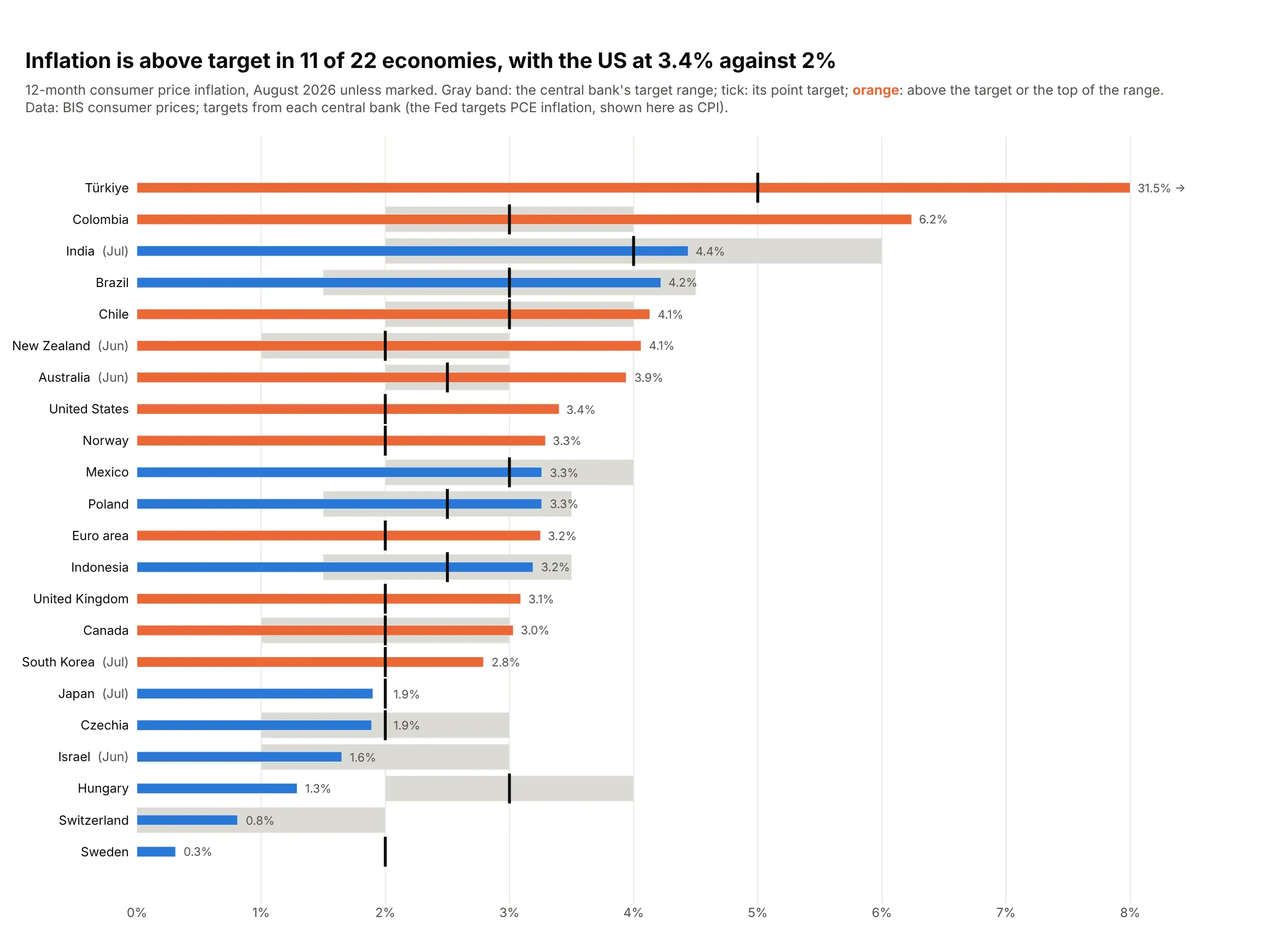
Data: BIS consumer prices, latest month to August 2026; targets from each central bank.
How do you read a bullet chart? In the example above, notice these things:
- Each row is one economy, and its thin bar is the latest 12-month consumer price inflation, drawn from a shared 0% line so the bar lengths compare directly.
- The black tick is the central bank's point target, like the Fed's 2% on the United States row, and the gray band is a target range, like Colombia's. Some economies have both, and Switzerland has only a band.
- Color gives the verdict so you don't have to compare each bar with its tick yourself: orange bars are above the target or the top of the range, and blue bars are inside it or below. Brazil and Chile have almost the same inflation, but Brazil is blue because its band reaches higher.
- Rows are sorted from the highest inflation to the lowest, so the biggest overshoots, Türkiye and Colombia, are at the top and the economies well below target, like Hungary and Sweden, are at the bottom.
- Watch the top row and the month labels. Türkiye's 31.5% runs off the axis, so its bar is cut at the edge and isn't drawn to scale, and the economies marked (Jun) or (Jul) show an older month than the August figures around them.
It's often used for charts like these:
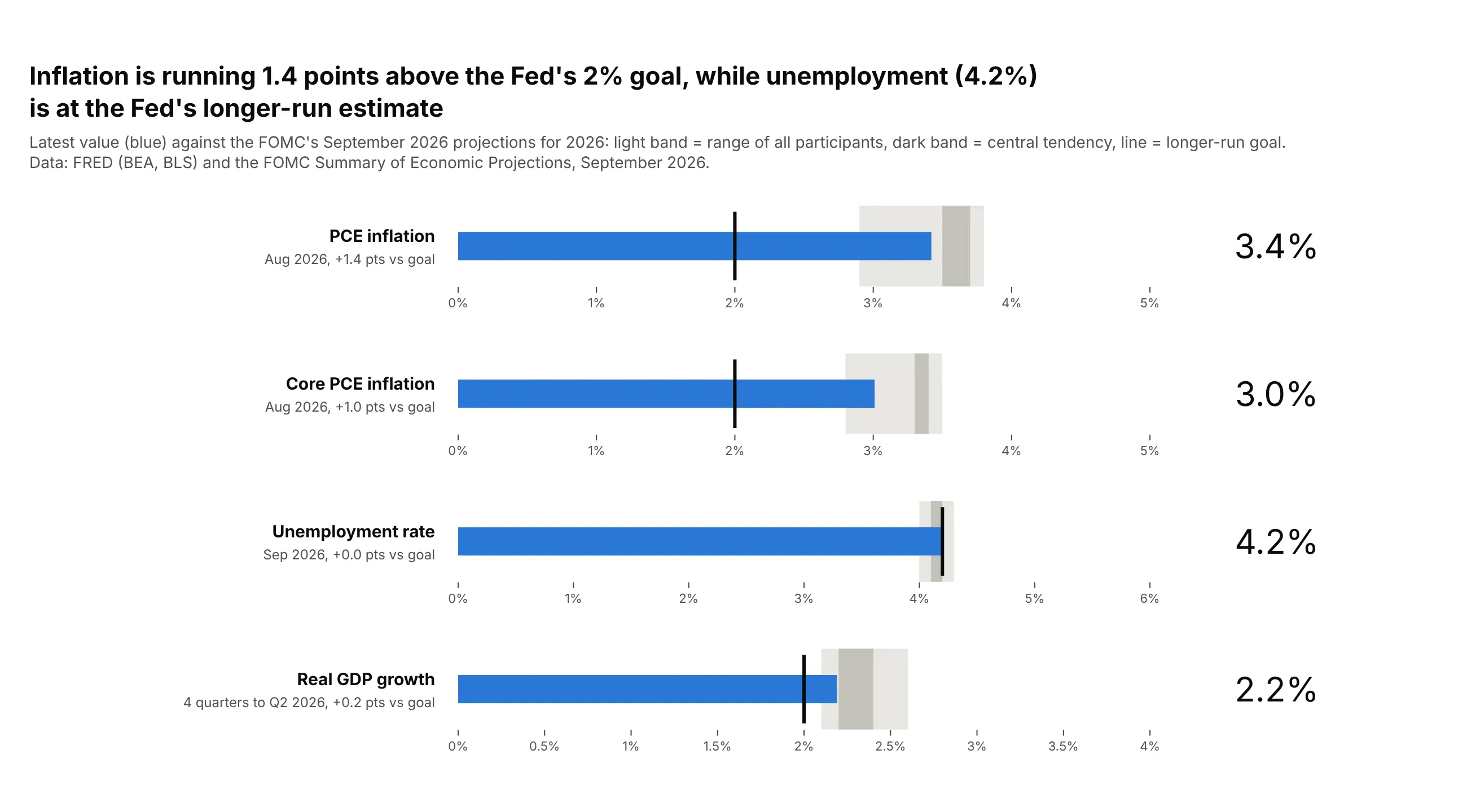
A KPI scorecard, each row on its own scale. US inflation was 1.4 points above the Fed's 2% goal in August 2026, while unemployment (4.2%) sat at the Fed's longer-run estimate. Data: FRED (BEA, BLS) and the FOMC Summary of Economic Projections, September 2026.
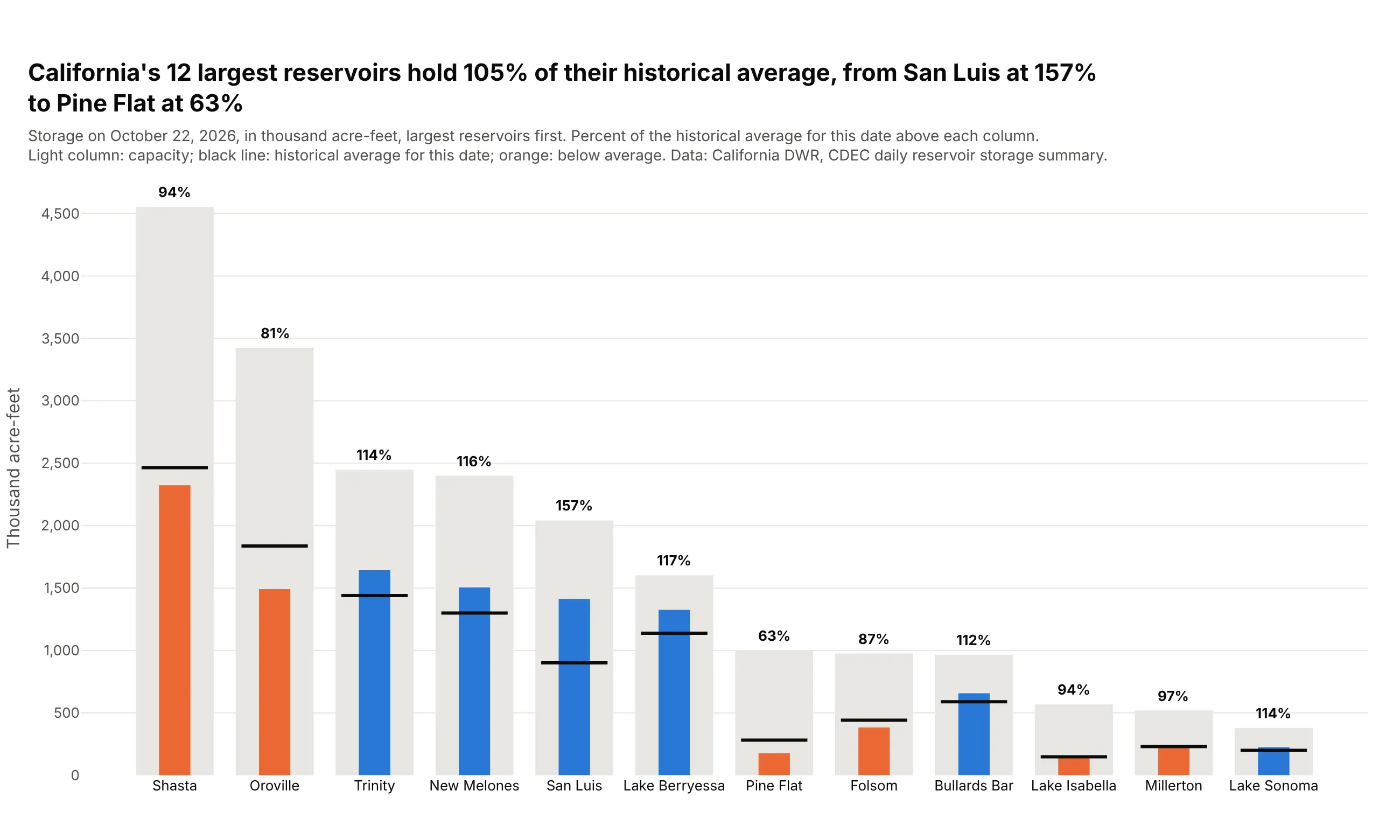
A level against capacity and its normal for the date. California's 12 largest reservoirs held 105% of their historical average, from San Luis at 157% to Pine Flat at 63%. Data: California DWR, CDEC daily reservoir storage summary, October 22, 2026.
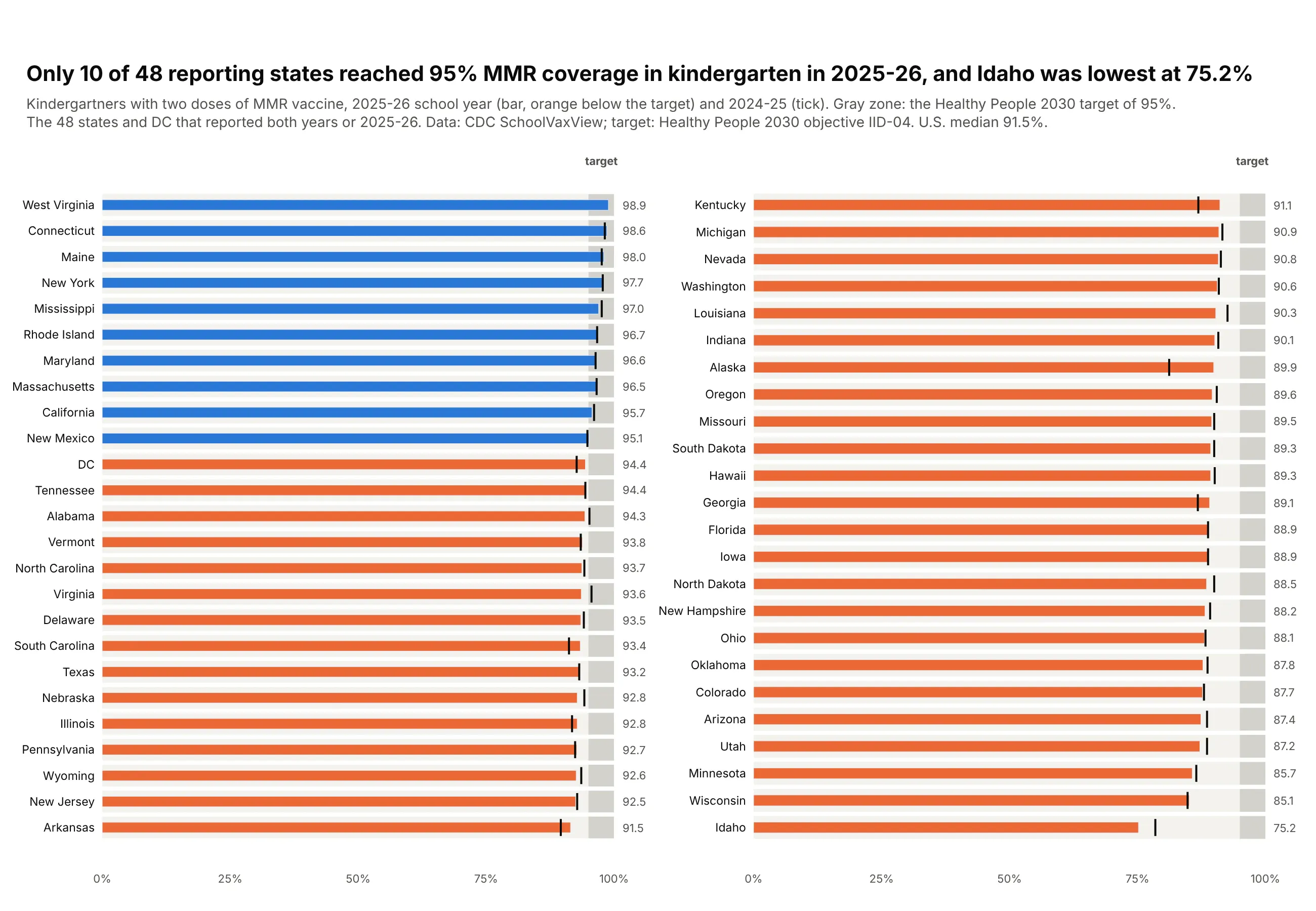
A long list against one target, compact like a table. Only 10 of 48 reporting states reached the 95% MMR target for kindergartners in 2025-26, and Idaho was lowest at 75.2%. Data: CDC SchoolVaxView; target from Healthy People 2030 objective IID-04.
A short history
Stephen Few developed the bullet graph to replace the meters and gauges on business dashboards, used it in Information Dashboard Design (O'Reilly, 2006), and published the Bullet Graph Design Specification (2006, last revised 2013) so software vendors could build it. This is a redraw with Plotly of his default design, a black bar a third as thick as the row and two to five ranges in shades of gray, on real data: JPMorgan Chase Bank's capital ratios in June 2026 against the regulators' four capital categories.
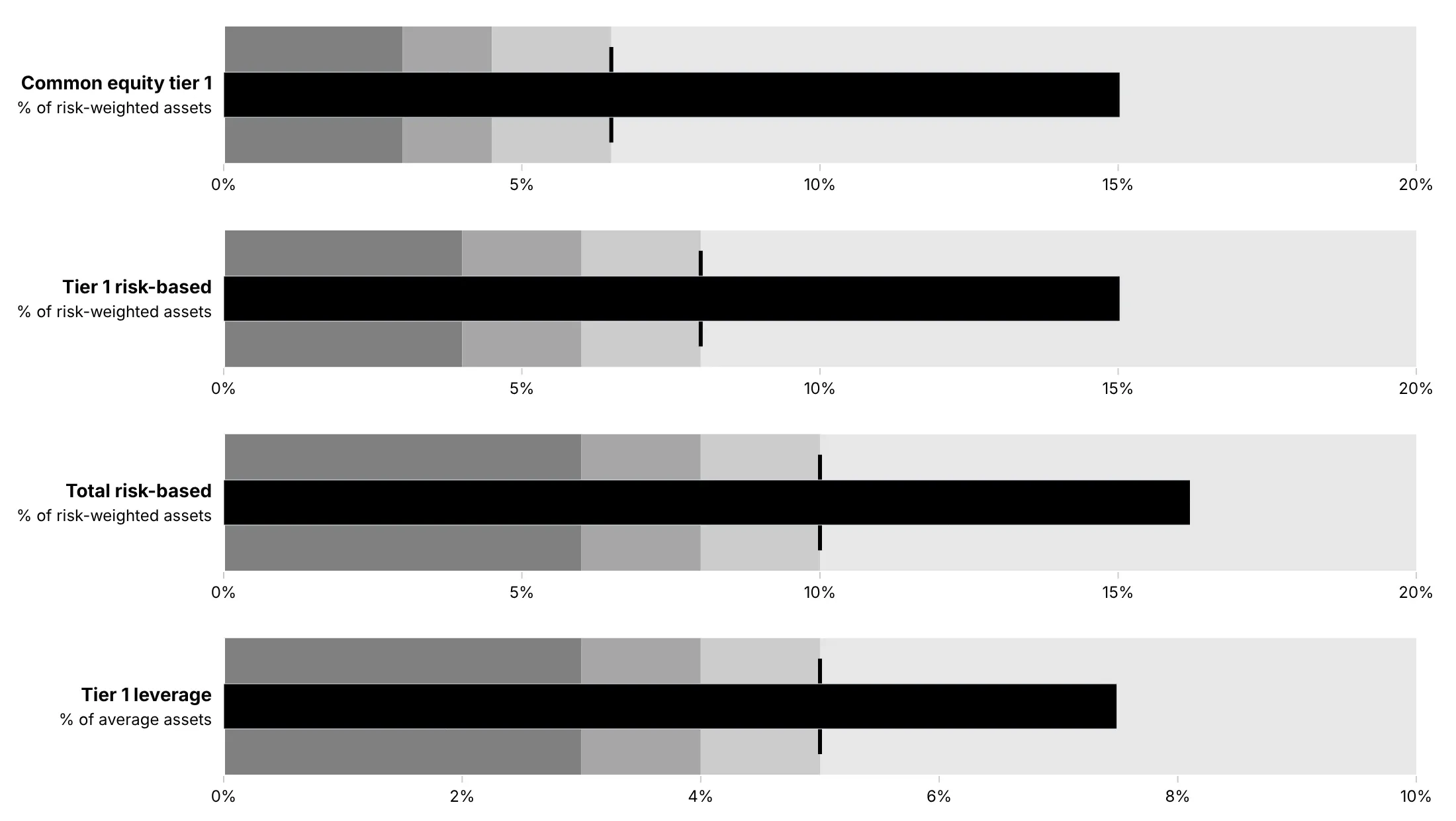
The design rests on the finding that people judge position and length along a common scale more accurately than angles or areas (Cleveland and McGill, 1984), which is why the value is a straight bar and not a needle.
Alternatives to a bullet chart
Here's the same set of four economic indicators drawn four ways. Some are better for the question, some worse, some just different:
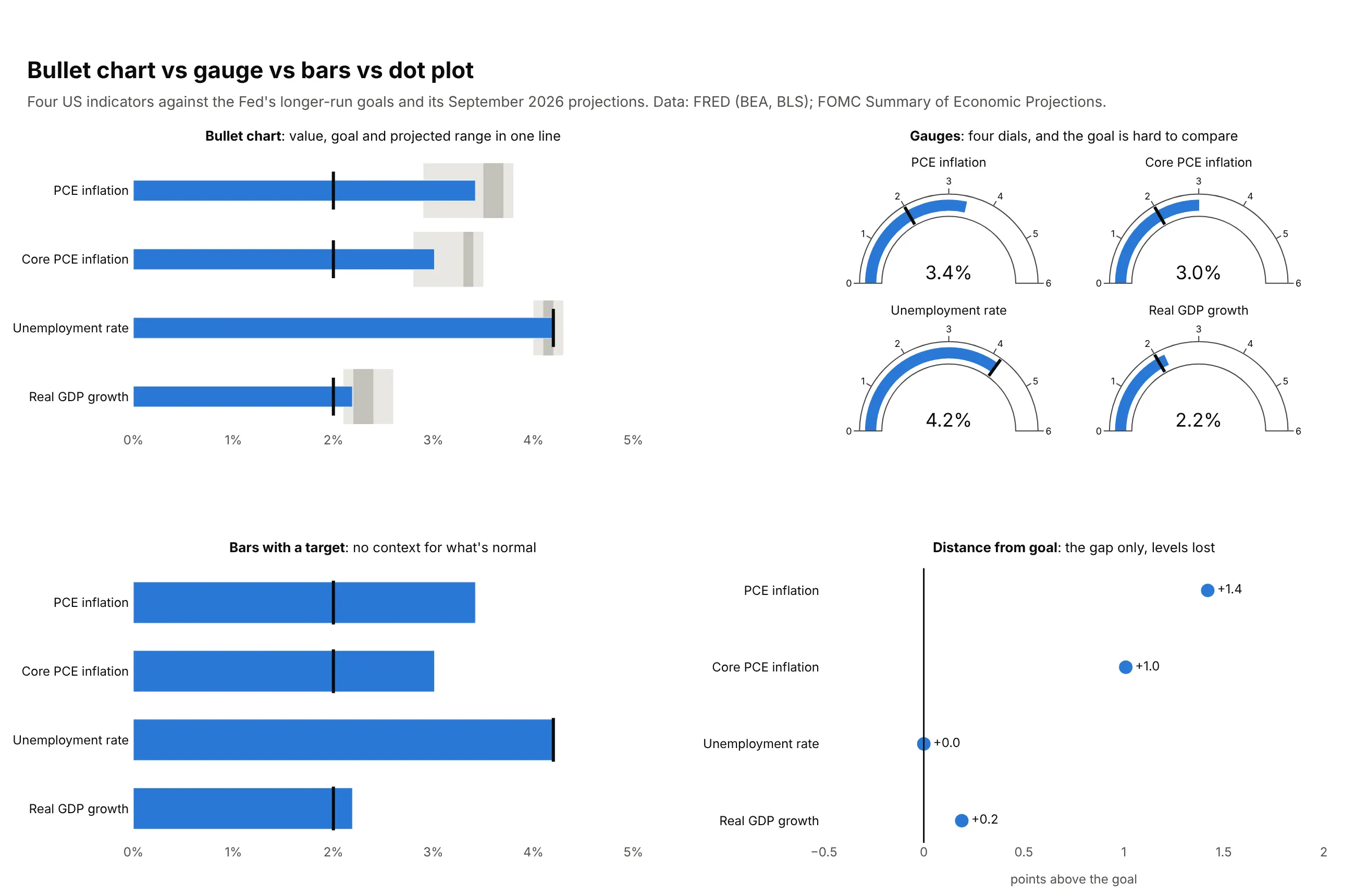
- Gauge (worse for comparing). One value per dial, a square of space each, and the goal is an angle that's hard to compare across dials. It still works for a single headline number on a wall display; see our gauge chart guide.
- Bar chart with a target line (works too, when there are no bands). Shows the value and the target, but not whether the value is normal or worrying.
- Distance from the goal (better when only the gap matters). A dot plot or diverging bar of value minus target ranks the misses clearly, but the level itself is gone.
- A big number with a change (different). A KPI card such as "3.4%, +1.4 pts" is the most compact of all, and loses the scale and the context the bands give.
How to make a bullet chart
With AI
ChatGPT, Claude Code, GitHub Copilot, Cursor and other AI tools are excellent at writing Plotly code. Name Plotly in the prompt, say what the target and the bands are, and list the checks you want:
Make a plotly bullet chart from kpis.csv (columns: team, metric, actual, target, poor_below, good_above).- One row per team, one panel per metric (make_subplots, shared y, each panel its own x axis).- Overlaid go.Bar traces, not go.Indicator: gray bands 0-poor_below, poor_below-good_aboveand good_above-max (darkest first), a thin blue bar for actual (width 0.3), and a blackline-ns marker for target.- Bars start at zero. Print the value after each bar. Color a bar orange only when it misses target.- A title that states the takeaway with a number, and a subtitle saying what the bands mean.- Assert poor_below < good_above for every row.- Save it as bullets.html and as a PNG at 2x scale.
With Plotly Studio
Plotly Studio is a desktop app where you point an AI at a dataset and it builds charts and a Dash app around your questions. Ask for a bullet chart the same way:
Show a bullet chart of each sales region's quarter-to-date revenue against its quota, with gray bands at 70% and 90% of quota and a black tick at the quota. Sort by percent of quota and add a dropdown to switch between revenue and gross margin.
Make a bullet chart in Python or JavaScript
This is the code AI tools write under the hood. You can make a bullet chart with any number of rows in Plotly from three kinds of traces: a go.Bar per range band (with base for where it starts), a thin go.Bar for the values and a go.Scatter with line-ns markers for the targets, drawn with barmode="overlay". This helper does it for any DataFrame, with a number or a column name for the target and each band:
import pandas as pdimport plotly.graph_objects as godef make_bullets(df, label, value, target=None, ranges=(), bar_color="#2a78d6",band_colors=("#c3c2bc", "#d4d2cb", "#e3e2dc", "#f3f2ee")):d = df.sort_values(value)col = lambda v: d[v] if isinstance(v, str) else pd.Series(v, index=d.index)fig, lo = go.Figure(), col(0)for r, color in zip(ranges, band_colors):fig.add_trace(go.Bar(y=d[label], x=col(r) - lo, base=lo, orientation="h",width=0.8, marker_color=color, hoverinfo="skip"))lo = col(r)fig.add_trace(go.Bar(y=d[label], x=d[value], orientation="h", width=0.3,marker_color=bar_color))if target is not None:fig.add_trace(go.Scatter(y=d[label], x=col(target), mode="markers",marker=dict(symbol="line-ns", size=22,line=dict(width=3, color="#0b0b0b"))))fig.update_layout(barmode="overlay", showlegend=False, template="simple_white")return figmmr = pd.read_csv("09_kindergarten_mmr.csv") # CDC SchoolVaxView, kindergarten MMR coveragefig = make_bullets(mmr, "state", "mmr_2025_26", target=95, ranges=[90, 95, 100])fig.show()
For a few KPIs, go.Indicator draws one bullet per trace in one line of code each:
import plotly.graph_objects as gofig = go.Figure(go.Indicator(mode="number+gauge", value=3.4, number={"suffix": "%"}, title={"text": "PCE inflation"},gauge={"shape": "bullet", "axis": {"range": [0, 5]},"steps": [{"range": [2.9, 3.8], "color": "#e8e7e2"}],"threshold": {"value": 2.0, "line": {"width": 3}}, "bar": {"thickness": 0.35}},))fig.show()
In JavaScript, plotly.js builds the same chart from the same three kinds of traces:
<div id="chart"></div><script src="https://cdn.plot.ly/plotly-4.1.1.min.js"></script><script>const states = ["Idaho", "Texas", "California"];const coverage = [75.2, 93.2, 95.7]; // kindergarten MMR, 2025-26 (CDC)const band = (from, to, color) => ({type: "bar", orientation: "h", y: states, base: states.map(() => from),x: states.map(() => to - from), width: 0.8, marker: {color}, hoverinfo: "skip"});Plotly.newPlot("chart", [band(0, 90, "#c3c2bc"), band(90, 95, "#dcdad3"), band(95, 100, "#efeee9"),{type: "bar", orientation: "h", y: states, x: coverage, width: 0.3, marker: {color: "#2a78d6"}},{type: "scatter", mode: "markers", y: states, x: [95, 95, 95],marker: {symbol: "line-ns", size: 22, line: {width: 3, color: "#0b0b0b"}}}], {barmode: "overlay", showlegend: false, xaxis: {range: [0, 100], ticksuffix: "%"}});</script>
For columns instead of rows, swap x and y and set orientation: "v" (as in the reservoir chart above).
Share it
Every Plotly chart has a Share chart button (the cloud icon in its toolbar) that uploads it to Plotly Cloud and gives you a link. Only you can see it until you change its visibility.
For a live app, put the chart in a Dash app and publish it with the Plotly Cloud CLI. Coding agents can run these commands for you:
pip install "dash[cloud]"plotly user loginplotly app publish
If your data has to stay in your own cloud or data center, publish to Dash Enterprise instead.
Dos and don'ts
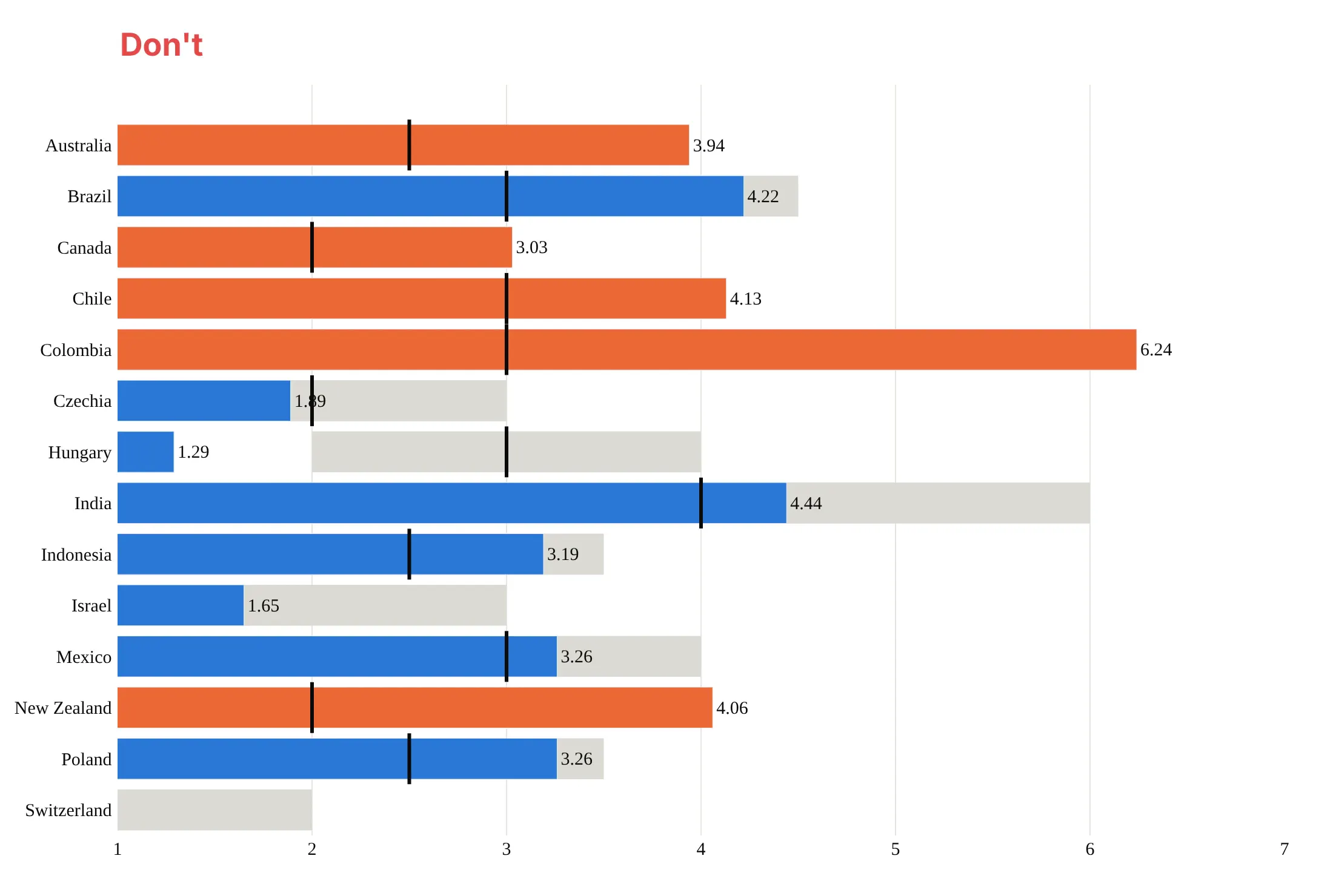
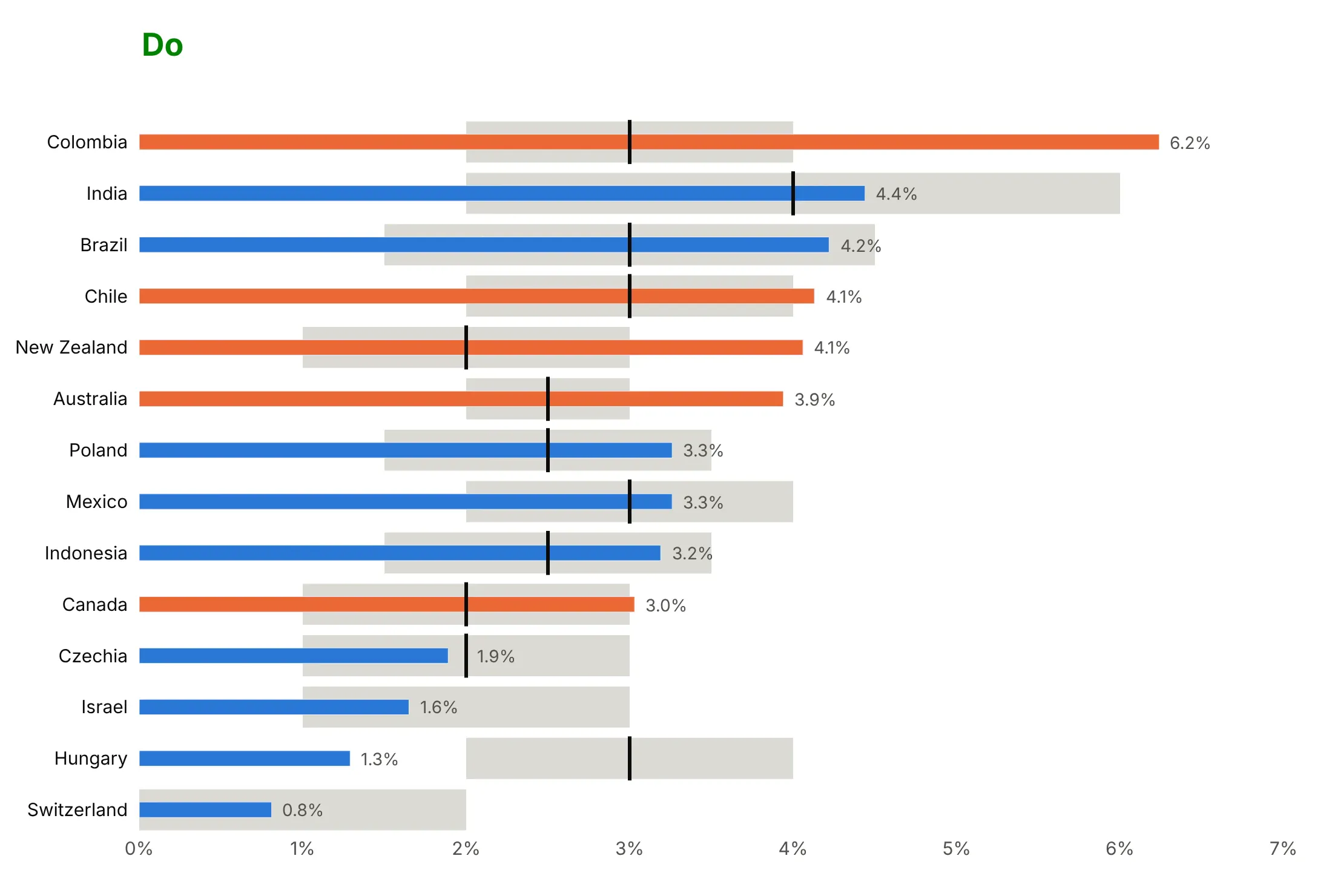
A bullet chart only works when the bands stay visible, the bars are honest and the rows are easy to scan. Here are the 14 economies with a target range from the inflation chart, drawn both ways with the same colors.
Don't sort the rows alphabetically, make the bar as thick as the band so the band disappears, start the axis at 1% so the bars' lengths lie (Switzerland's 0.8% vanishes), or print raw numbers like 4.06 in a serif font:
Do sort the rows, keep the bar about a third of the band's height, start the axis at zero and label each bar with a rounded value:
Bands and markers
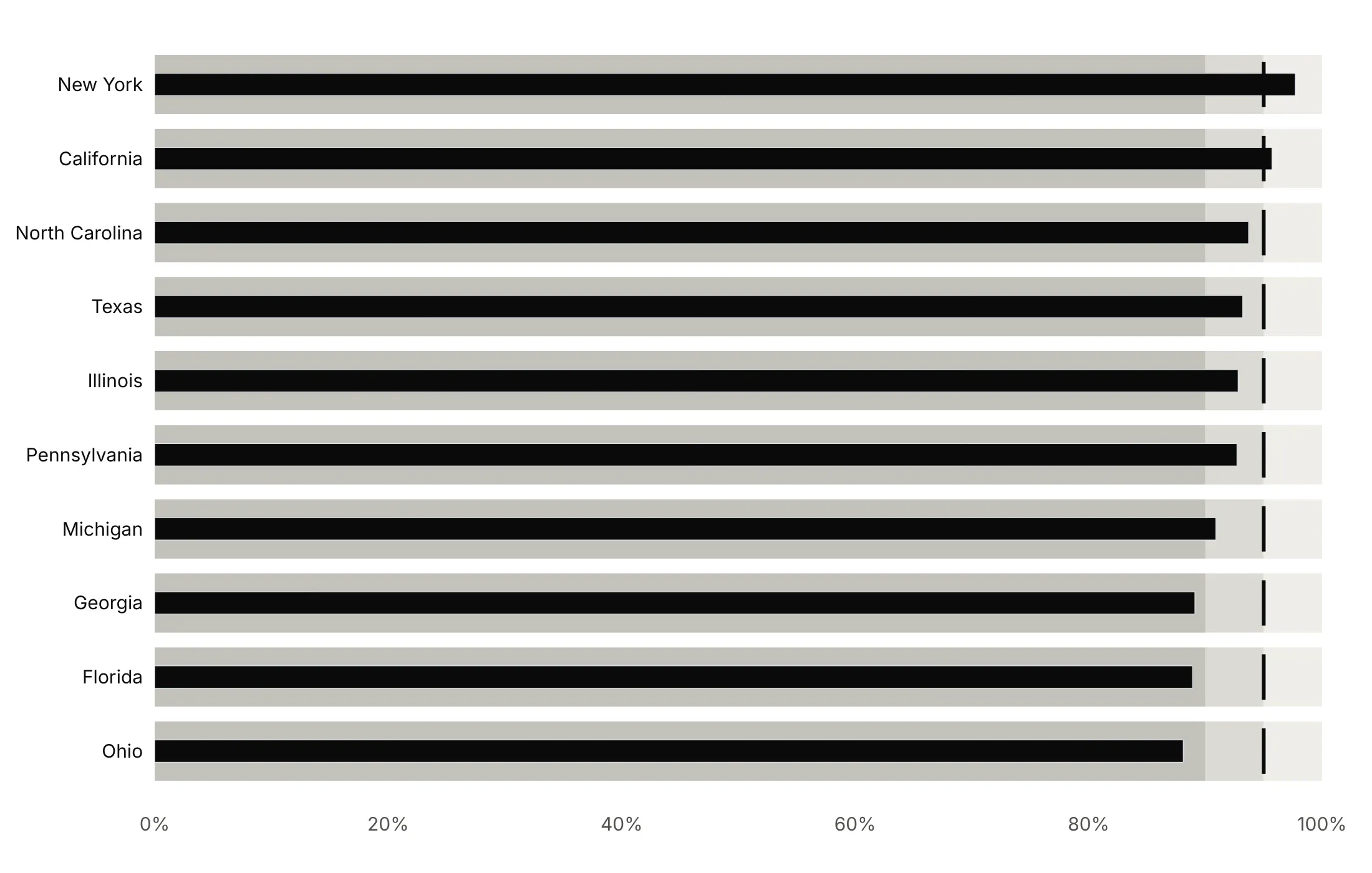
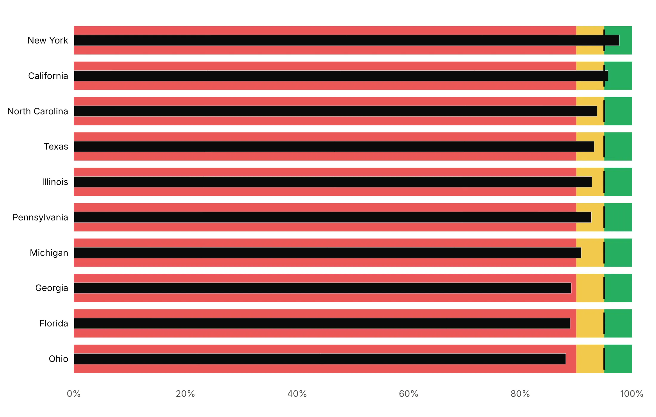
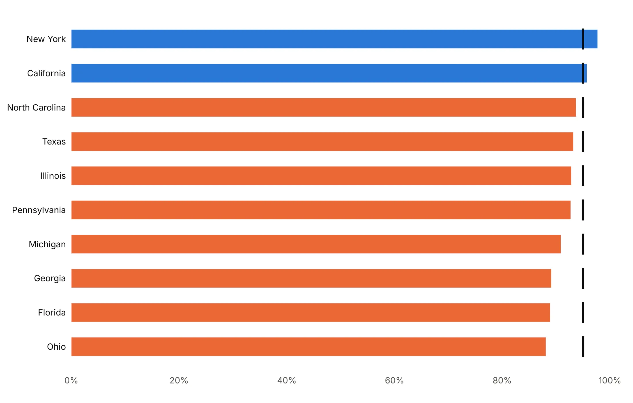
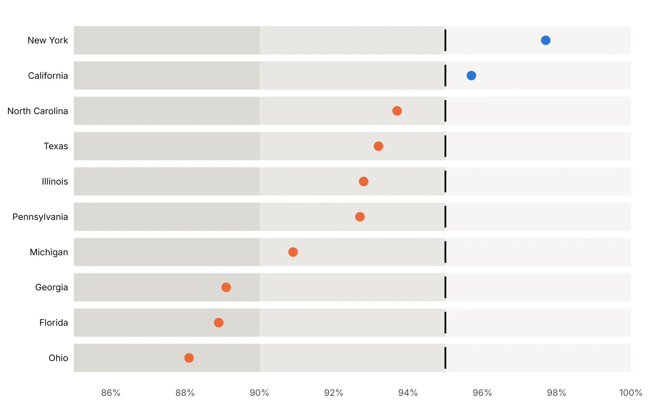
Here are four ways to style the same kindergarten MMR coverage in the 10 most populous states against the 95% target.
Gray ranges, a dark bar and a target tick. Stephen Few's default, readable in grayscale and for color-blind readers.
Traffic-light ranges (avoid). Red, yellow and green bands are loud, pull the eye away from the bars and fail for red-green color blindness.
No ranges, the bar colored by status. Simpler when there is only a target, with blue for the two states at or above 95% and orange for the eight below.
A dot on a zoomed axis. When the interesting range is 85-100%, a bar would lie about its length, so the value becomes a dot, as Few's specification recommends.
Checklist
Do
- Write a title that states the takeaway, and say what the bands mean in the subtitle.
- Keep the bar thin and the bands in two to five shades of one gray, darkest for worst.
- Draw the target as a short dark line, and sort the rows.
- Print the value after each bar.
- Give each row its own axis when the units differ, or convert to percentiles to share one.
- Clip a single outlier at the edge of the axis and print its true value.
Don't
- Start a bar anywhere but zero; use a dot on a zoomed axis instead.
- Use red, yellow and green bands.
- Use more than five bands.
- Use one go.Indicator per row for long lists; overlaid bars are much faster.
Options to customize
These are the options that matter for both ways of building a bullet chart. The full lists are in the Plotly bullet chart documentation, the indicator reference and the bar reference.
- go.Indicator(gauge_shape="bullet"): one bullet per trace, for scorecards of up to about 10 KPIs.
- gauge.steps: the qualitative bands, each {"range": [a, b], "color": ...}.
- gauge.threshold: the target line, with value, line.width and thickness.
- gauge.bar.thickness: the bar's height as a share of the gauge; about 0.3 keeps the bands visible.
- gauge.axis.range: the scale of one bullet, so each KPI can have its own.
- domain: where each indicator sits, for stacking several.
- mode: "gauge", "number" and "delta" in any combination, to add the big number or a change.
- go.Bar(base=...): where a bar starts, for bands that don't start at zero.
- go.Bar(width=...): bar height in category units; 0.8 for bands, 0.3 for the value.
- layout.barmode="overlay": draws the bands and the value bar on top of each other.
- marker.symbol="line-ns" or "line-ew": a short line marker for targets; it needs marker.line.width.
- orientation: "h" for rows or "v" for columns.
- make_subplots(shared_yaxes=True): panels with their own x axes, for several measures per row or a long list split in two.
- xaxis.range: the axis limits; clip one outlier and print its value.
- go.Scatter(mode="markers"): a dot instead of a bar, for axes that don't start at zero.
- hovertemplate, customdata: hover text with the unclipped value or the target.
More bullet chart examples
Seven more bullet charts built from real public data, each with its source, the technique that makes it work and a prompt to rebuild it.
1. The largest US banks against regulatory capital thresholds
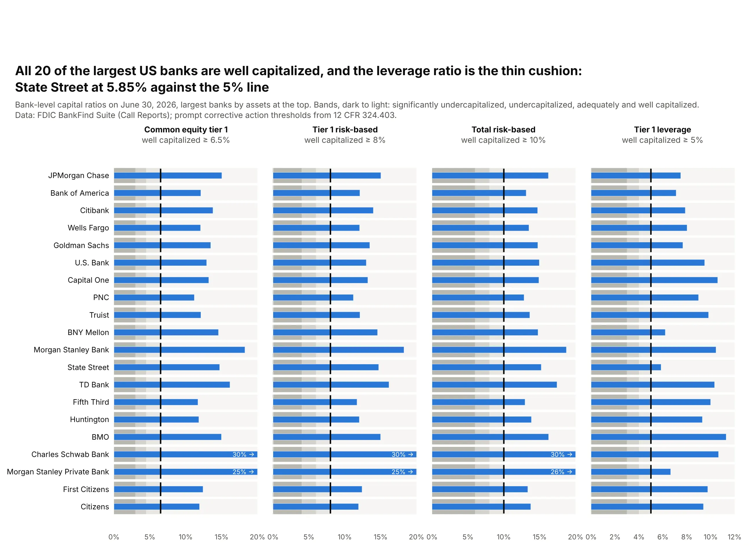
All 20 of the largest US banks are well capitalized on all four ratios. The cushion is thinnest on the tier 1 capital to assets ratio, where State Street is at 5.85% against a 5% line and BNY Mellon at 6.20%. Risk-based ratios sit far above theirs, from 11.2% upward. Data: FDIC BankFind Suite (Call Reports), June 30, 2026; thresholds from 12 CFR 324.403.
Tip: make_subplots(cols=4, shared_yaxes=True) gives each ratio its own thresholds and axis while the banks line up across all four panels.
Get the data from the FDIC BankFind Suite API (api.fdic.gov/banks/financials) for the quarterending 2026-06-30, the 20 largest banks by assets, and shape it into a table(columns: bank, assets_bn, cet1, tier1, total, leverage; ratios in percent).Build a 4-panel plotly bullet chart (make_subplots, shared y), largest bank at the top.- Bands from 12 CFR 324.403: significantly undercapitalized, undercapitalized, adequately andwell capitalized (CET1 3/4.5/6.5, tier 1 4/6/8, total 6/8/10, leverage 3/4/5), darkest first.- Thin blue bar for the ratio, a black tick at the well-capitalized line.- Axis 0-20% (0-12% for leverage); clip larger values and print them in white inside the bar.- Title naming the bank closest to any threshold.
2. EU countries against the Maastricht limits
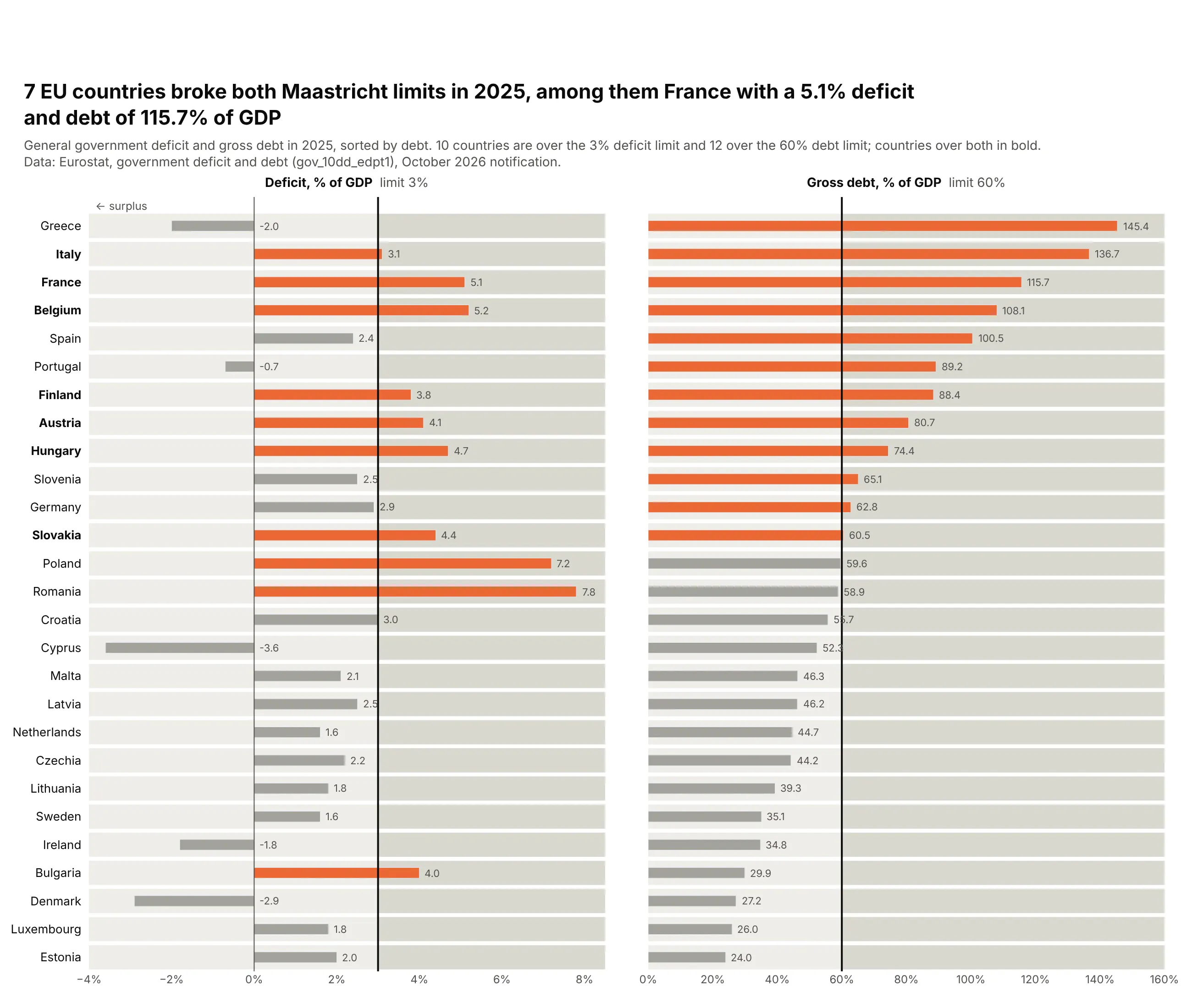
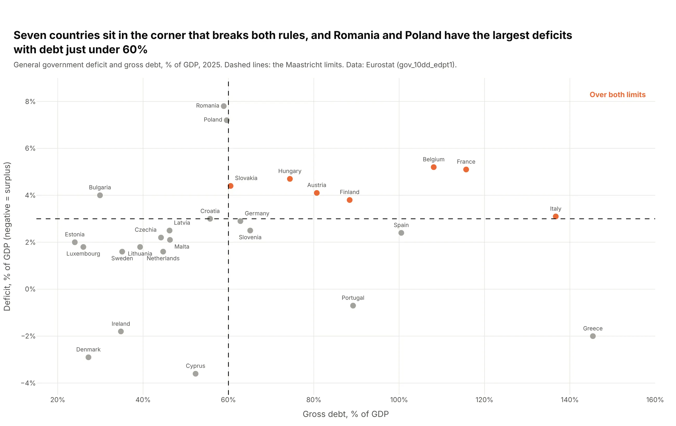
A legal limit splits each axis into "within" and "over", the simplest qualitative range. Ten countries ran deficits above 3% of GDP in 2025, 12 had debt above 60%, and seven broke both, among them France (5.1% and 115.7%). Data: Eurostat government deficit and debt (gov_10dd_edpt1), 2025.
Tip: a two-tone background (base=limit for the darker half) shows the limit even where no bar reaches it, and surpluses run left of a zero line.
Get the data from Eurostat's government deficit and debt dataset (gov_10dd_edpt1, % of GDP,general government) for 2025, and shape it into a table(columns: country, deficit (positive = deficit), debt; the 27 EU members).Build a 2-panel plotly bullet chart sorted by debt: deficit (axis -4 to 8.5%) and debt (0-160%).- Light band up to the limit (3% and 60%), slightly darker band beyond it, black line at the limit.- Bar orange where over the limit, gray otherwise; value printed after each bar.- Bold the names of countries over both limits; title with that count.
Another way to see it: a scatter of debt against deficit puts the seven countries over both limits in one corner, and shows Romania (7.8%) and Poland (7.2%) with the largest deficits but debt just under 60%.
3. US natural gas storage against its five-year range
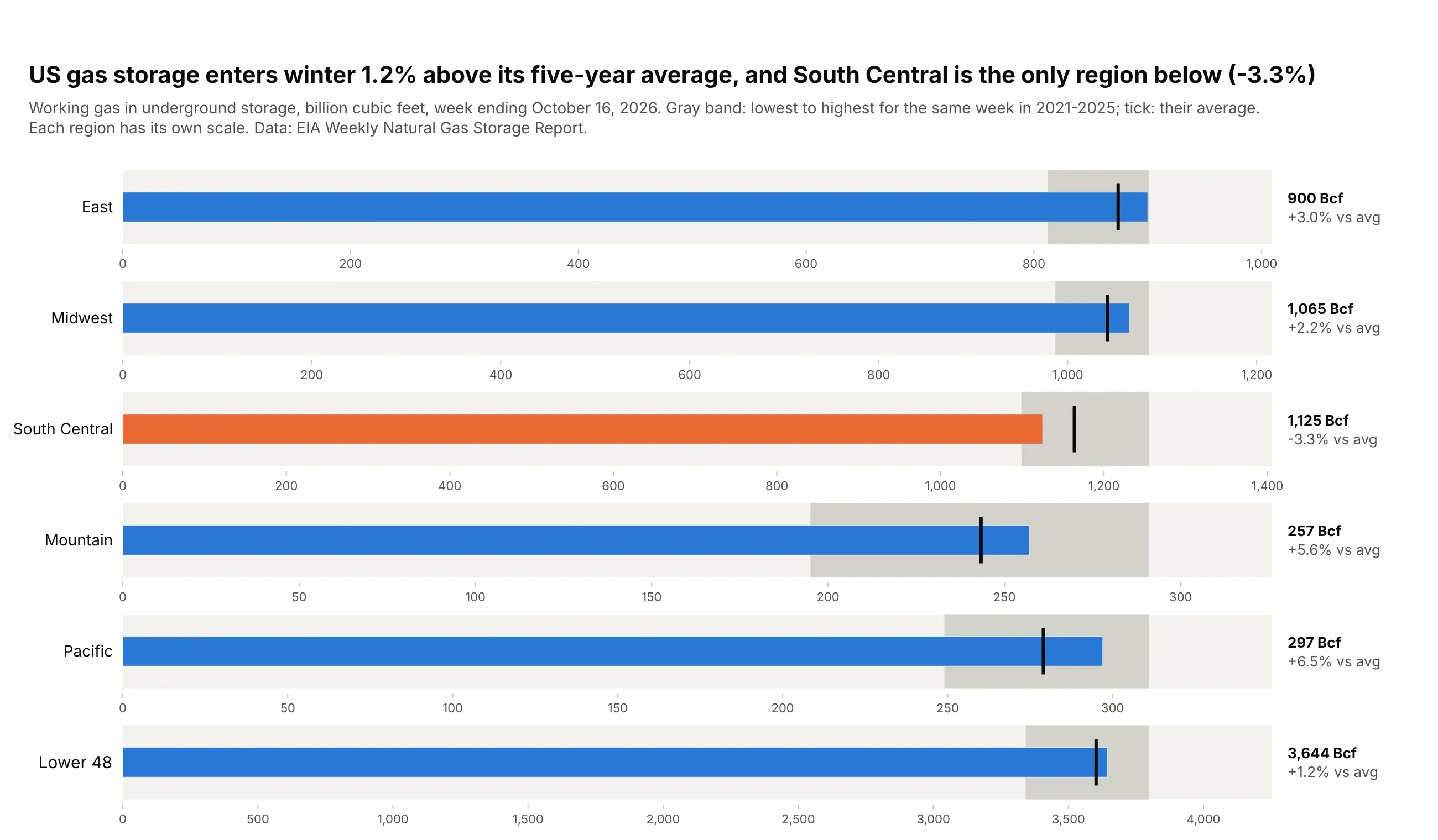
The five-year low-to-high range is the band and the five-year average the tick. US storage entered winter at 3,644 Bcf, 1.2% above average, and South Central was the only region below it (-3.3%). Data: EIA Weekly Natural Gas Storage Report, week ending October 16, 2026.
Tip: South Central holds 4.4 times as much gas as Mountain, so make_subplots(rows=6) gives every region its own x axis, as in Few's original design.
Get the data from the EIA Weekly Natural Gas Storage Report history (eia.gov, working gas inunderground storage by region, Bcf), and shape it into a table(columns: region, week, storage_bcf, avg5, min5, max5; the five-year values are the same week ineach of the previous five years).Build a plotly bullet chart with make_subplots(rows=6), one region per row, each with its own x axis from 0.- Light background to 112% of max5, darker band from min5 to max5, black tick at avg5.- Bar blue if above avg5, orange if below. Print "1,125 Bcf / -3.3% vs avg" to the right.- Title with the Lower 48 vs average and the regions below it.
4. EU countries against their 2020 renewable energy targets
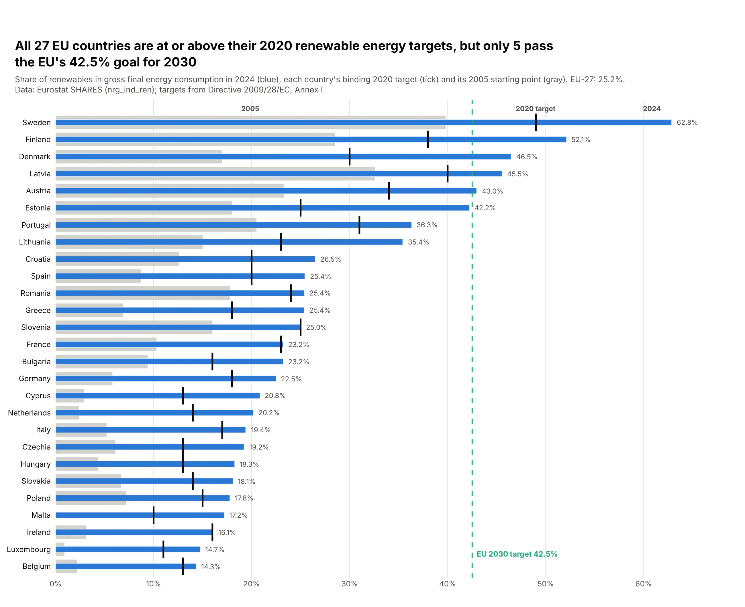
Each country had its own binding target for 2020, and the gray band shows where it started in 2005. In 2024 all 27 were at or above their 2020 targets, but only five passed the EU's 42.5% goal for 2030. Data: Eurostat SHARES (nrg_ind_ren), 2024; targets from Directive 2009/28/EC, Annex I.
Tip: the band can be a comparative value rather than a quality range: here it is the 2005 share, so the bar's overhang is progress.
Get the data from Eurostat SHARES (nrg_ind_ren, renewable share of gross final energyconsumption) for 2024, and the national 2020 targets and 2005 shares in Annex I ofDirective 2009/28/EC, and shape it into a table(columns: country, share_2005, target_2020, share_2024).Build a plotly bullet chart sorted by share_2024.- Gray bar from 0 to share_2005, thin blue bar for share_2024, black tick at target_2020.- Dashed green vertical line at the EU 2030 target of 42.5% with a label.- Label "2005", "2020 target" and "2024" above the top row instead of a legend.
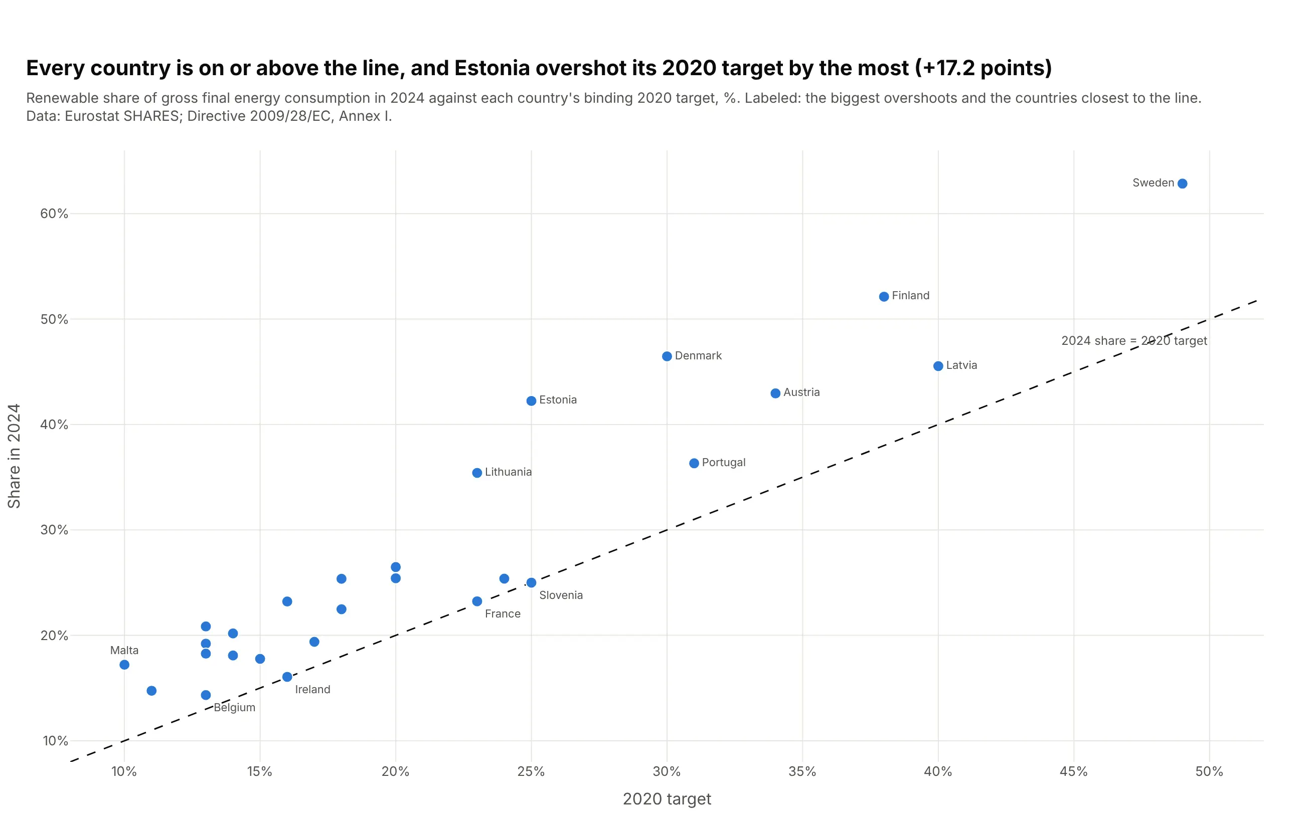
Another way to see it: a scatter of target against result puts every country above the diagonal and shows Estonia overshooting the most (+17.2 points).
5. Fine particle pollution in large US metros against EPA and WHO limits
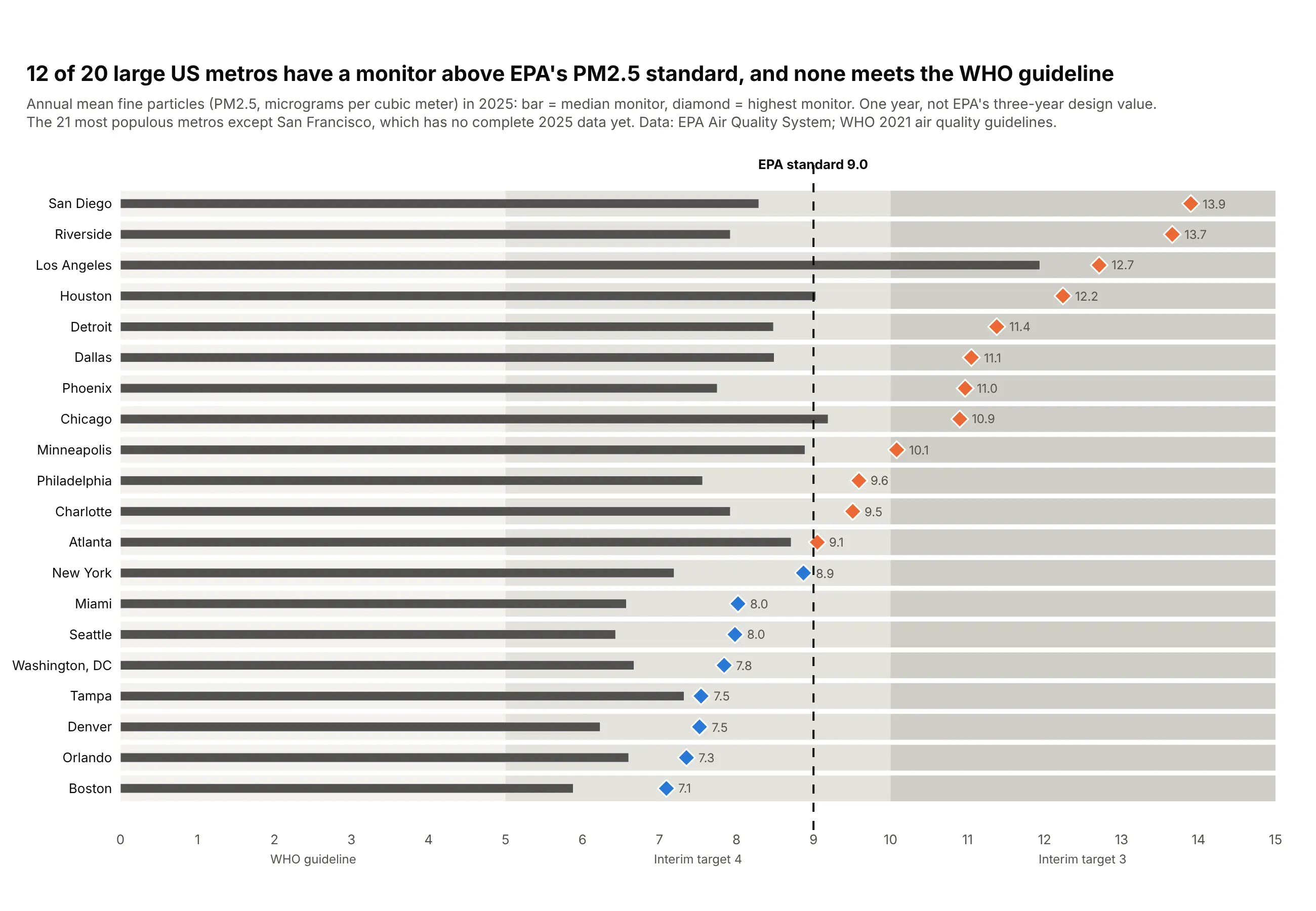
The WHO guideline and interim targets are the bands, and a diamond adds the worst monitor to the typical one. Twelve of 20 large metros had a monitor above EPA's 9.0 µg/m³ standard in 2025, and none met the WHO guideline of 5. Data: EPA Air Quality System annual summaries, 2025; WHO 2021 air quality guidelines.
Tip: a second marker per row (symbol="diamond") shows a spread, the typical and the worst value, without a second chart.
Get the data from the EPA Air Quality System annual summary by monitor for 2025(aqs.epa.gov/aqsweb/airdata, PM2.5 parameter 88101, annual standard, complete data),with metro populations from the Census Bureau, and shape it into a table(columns: metro, sites, median_site, max_site; µg/m³; 20 large metros).Build a plotly bullet chart sorted by max_site.- Bands for the WHO guideline (0-5), interim target 4 (5-10) and 3 (10-15), lightest first.- Dark gray bar for median_site; diamond for max_site, orange above 9.0, blue otherwise.- Dashed black line at EPA's 9.0 standard; band names under the axis.- Subtitle says this is one year, not a three-year design value.
6. Heart failure readmissions against each hospital's expected rate
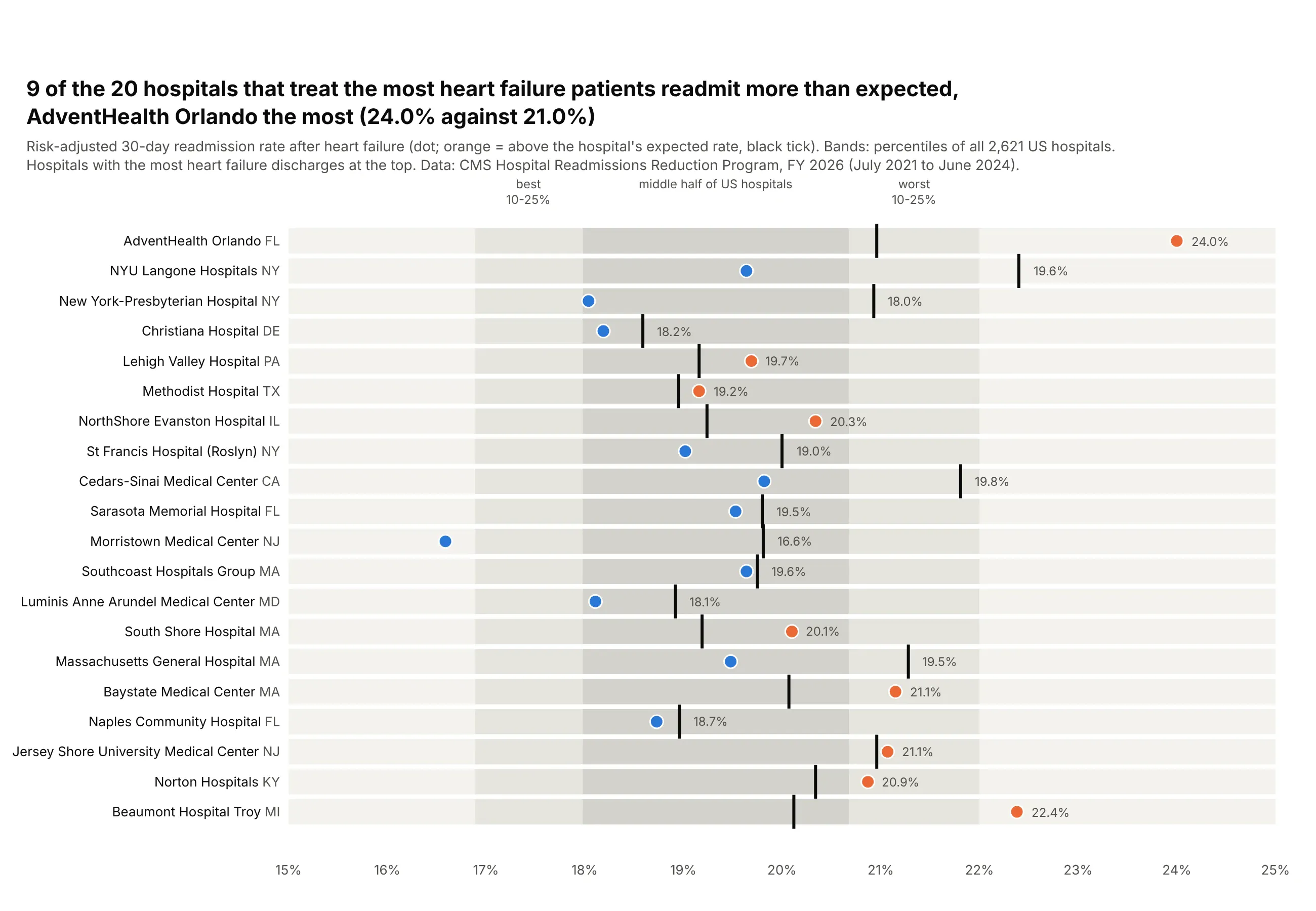
Each hospital's target is different, the rate expected for its own patients, and the bands are the national percentiles. Nine of the 20 busiest hospitals readmitted more heart failure patients than expected, AdventHealth Orlando the most (24.0% against 21.0%). Data: CMS Hospital Readmissions Reduction Program, FY 2026.
Tip: the axis starts at 15%, so the value is a dot (go.Scatter) instead of a bar.
Get the data from the CMS Hospital Readmissions Reduction Program FY 2026 file(data.cms.gov provider data, measure READM-30-HF-HRRP), and shape it into a table(columns: hospital, state, discharges, predicted, expected, err) for the 20 hospitals with themost discharges, plus the 10th, 25th, 75th and 90th percentiles of predicted across all hospitals.Build a plotly bullet chart with an x axis from 15% to 25%.- Bands from the national percentiles (middle half darkest), labeled above the plot.- Dot for predicted, orange if err > 1, blue otherwise; black tick for expected.- Rows by discharges, largest at the top; the state in muted text after the name.
7. Shohei Ohtani's 2026 season against every qualified hitter
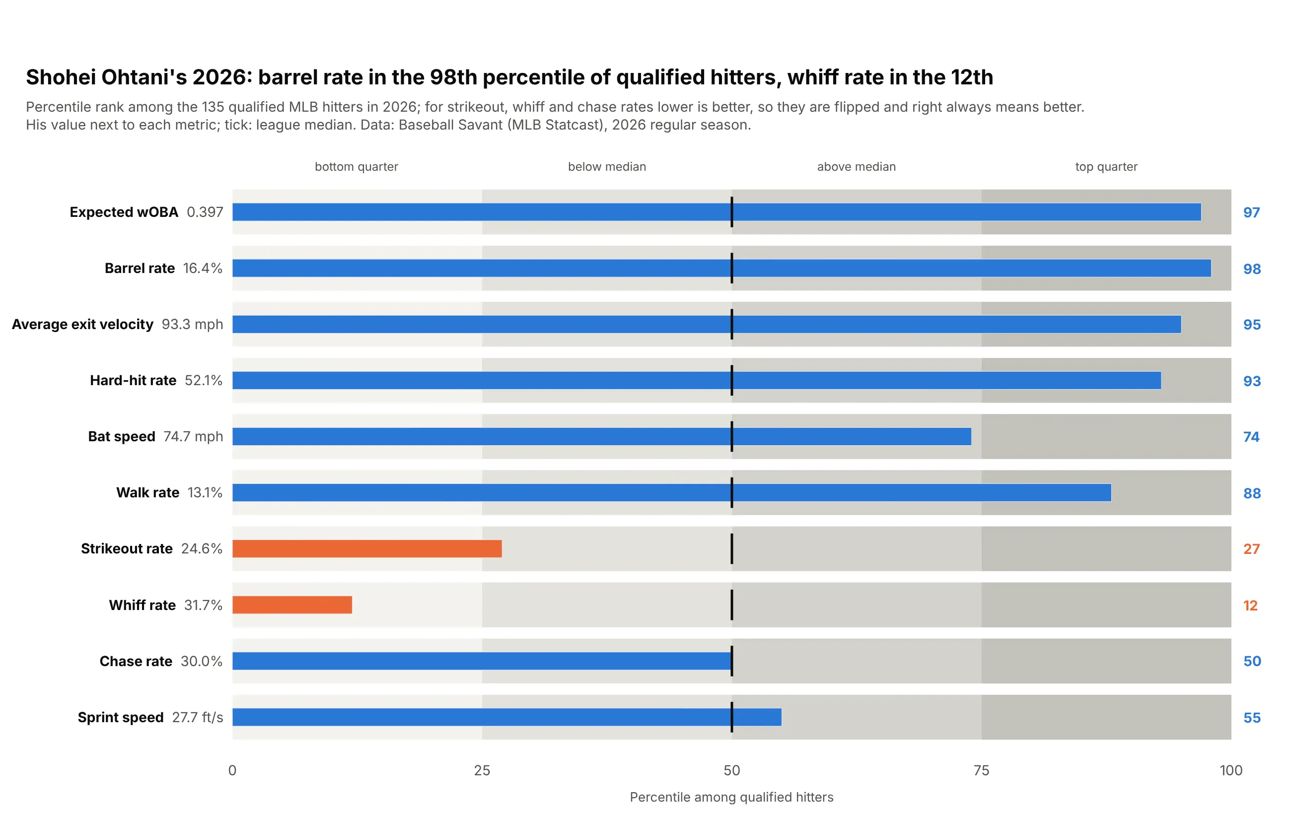
Ten metrics in mph, ft/s and percentages share one axis once each becomes a percentile among the 135 qualified hitters. Shohei Ohtani ranked in the 98th percentile for barrel rate but the 12th for whiff rate. Data: Baseball Savant (MLB Statcast), 2026 regular season.
Tip: flip lower-is-better metrics before ranking, so the right side always means better.
Get the data from the Baseball Savant custom leaderboard (MLB Statcast) for 2026 qualifiedhitters, and shape it into a table(columns: player, xwoba, barrel_pct, exit_velocity, hard_hit_pct, bat_speed, bb_pct, k_pct,whiff_pct, chase_pct, sprint_speed).Build a plotly bullet chart for one player.- Convert each metric to his percentile among all qualified hitters; for k_pct, whiff_pct andchase_pct, lower is better, so rank them the other way.- Quartile bands (0-25-50-75-100), lightest to darkest, a black tick at 50.- Bar blue at or above 50, orange below; percentile printed at the right, the raw valuenext to the metric name.