
Chris Parmer
November 20, 2026
Methane venting and flaring monitoring app
A data app example built with Dash and an AI coding agent in 40 minutes
TL;DR
- Building data apps with AI coding agents in Python and managing them on Dash Enterprise or Plotly Cloud is the modern alternative to BI. At Plotly, many of our customers are migrating away from point-and-click tools like Spotfire, Tableau, and Power BI toward code-backed tools powered by AI. This example showcases the types of apps that you can create.
- This app maps the natural gas that operators vent and flare across New Mexico's side of the Permian Basin, from the state's public monthly reports, next to every well, the major US gas pipelines, and NASA satellite methane plumes. A coding agent built it from one prompt in about 40 minutes.
- About 100,000 wells and EIA's map of US gas pipelines are drawn as vector tiles that DuckDB builds, so the map stays fast from the whole basin down to a single well pad.
- You can click any reporting site to open its own page with its monthly history, the wells around it, and the nearest pipeline.
- The full prompt is below, so you can build the same kind of app on your own data and run it on Dash Enterprise behind your firewall or have it hosted for you on Plotly Cloud.
Walkthrough
Methane is the gas emissions teams, regulators, and investors are watching most closely in oil and gas, and in New Mexico every operator reports the gas it vents and flares, well by well, every month. This app puts those reports on one map with the wells, the pipelines, and what NASA's EMIT instrument saw from the International Space Station.
It covers New Mexico only. Each reporting site has its own page and URL, so a link to a tank battery opens that tank battery.
See every well, pipeline, and venting site on one map
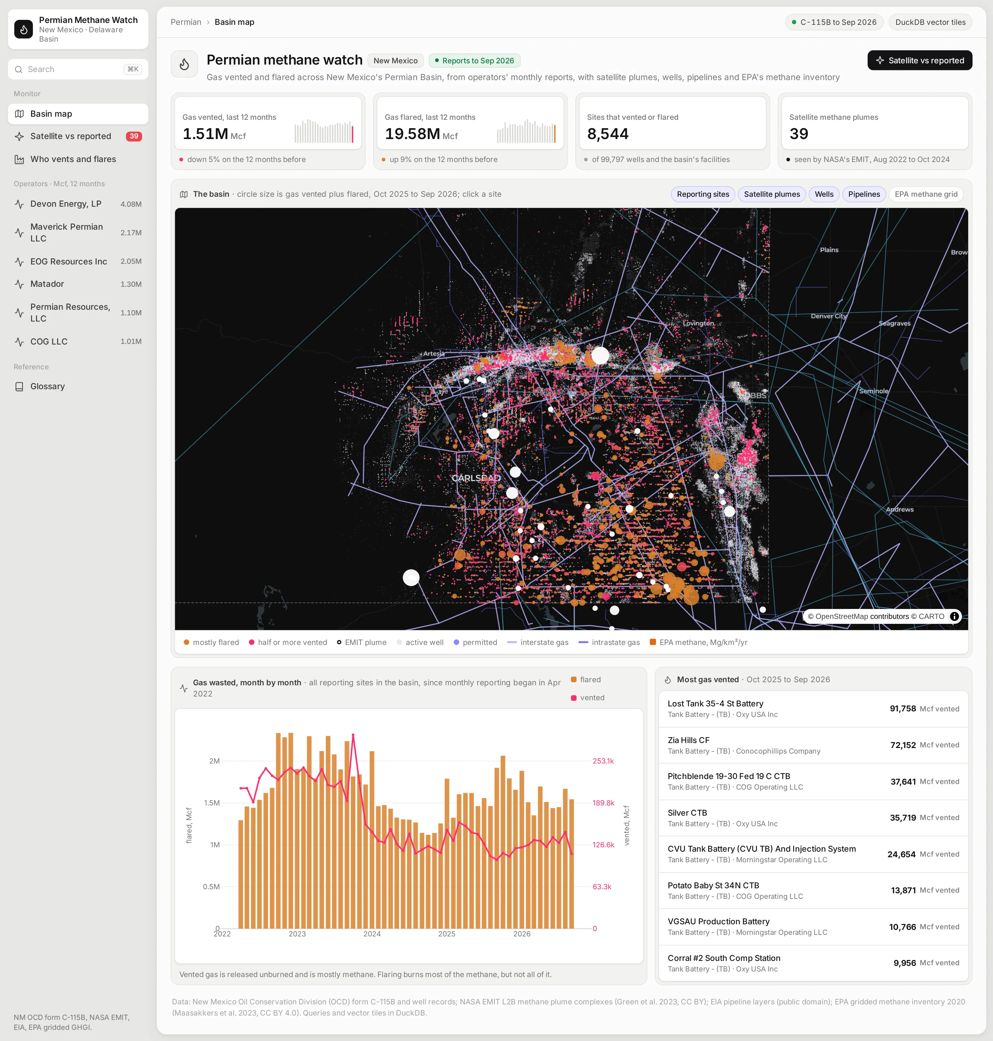
The basin page answers the first questions anyone asks: how much gas was vented and flared over the last 12 months, whether that's going up or down, and where it happened. Each reporting site is a circle sized by its volume, and its color shows whether most of its gas was flared or vented.
Venting matters more for methane, because the gas goes into the air unburned. Buttons on the map turn each layer on and off, including EPA's gridded methane inventory.
Zoom from the basin to a single well pad
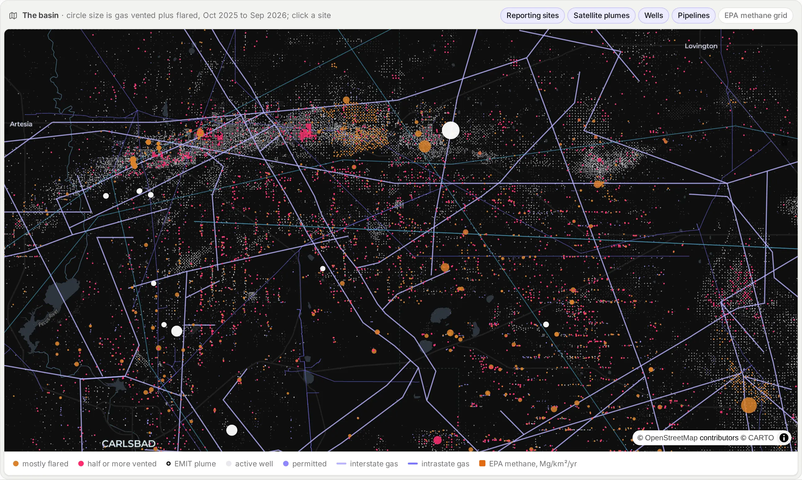
The wells and pipelines are vector tiles: small binary tiles of map data for each zoom level, which the browser draws with Plotly's map. DuckDB's spatial extension builds each one with a query like this (simplified), and the data prep step stores about 79,000 of them in a table in the app's DuckDB file:
SELECT ST_AsMVT(t, 'wells_active', 4096) FROM (SELECT api, ST_AsMVTGeom(geom, ST_Extent(ST_TileEnvelope(z, x, y)), 4096, 8, true) AS geomFROM wells WHERE state = 'active' AND <the tile's bounding box>) AS t
When the map asks for a tile, a Flask route on the Dash server reads it from that table:
@server.route("/tiles/<layer>/<int:z>/<int:x>/<int:y>.pbf")def tiles(layer, z, x, y):body = tile(layer, z, x, y) # stored gzippedreturn Response(body, mimetype="application/x-protobuf", headers={"Content-Encoding": "gzip"})
That's enough to keep about 100,000 wells and EIA's interstate and intrastate gas pipelines fast at any zoom, with no tile server to run.
Check satellite plumes against what operators reported
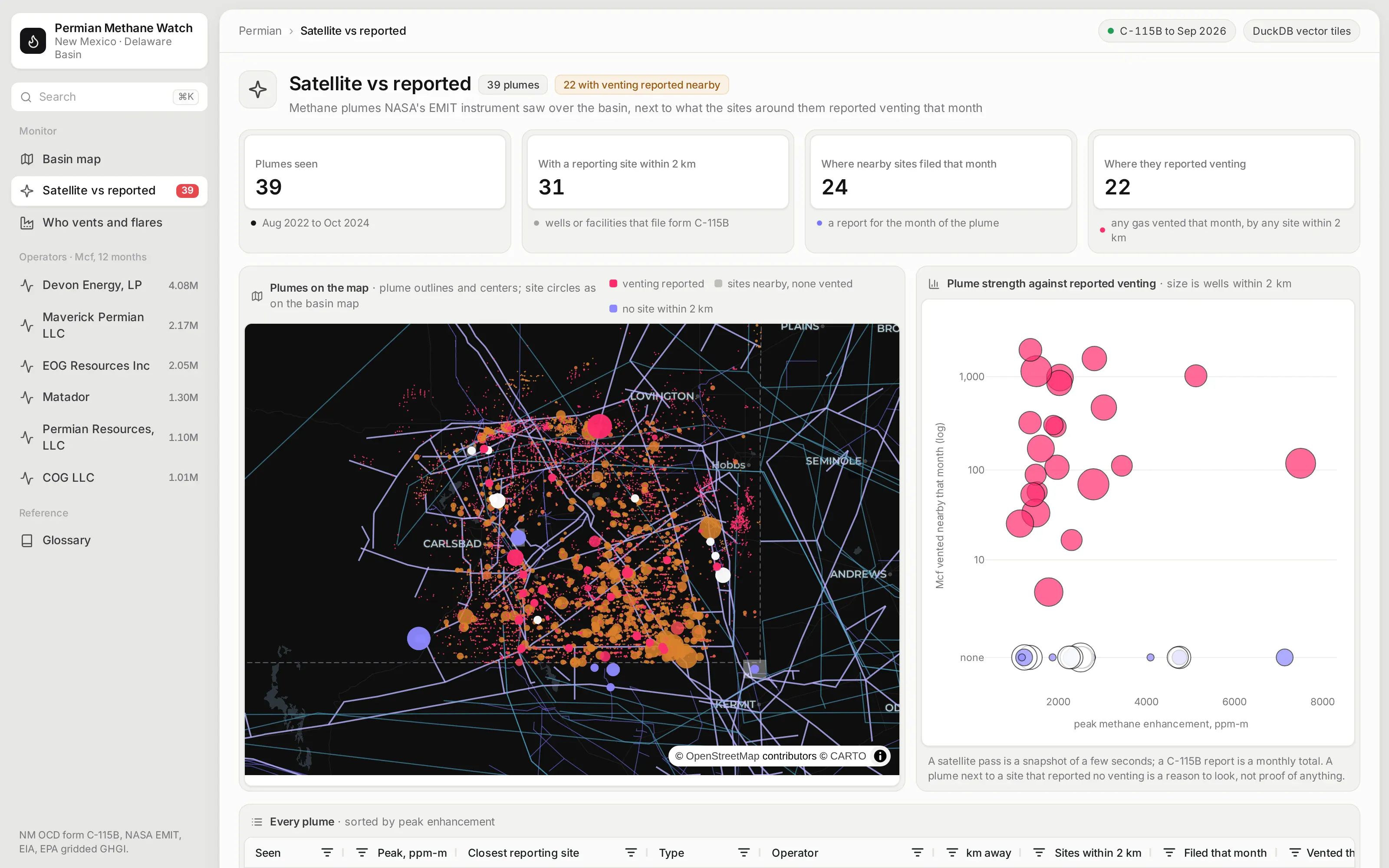
NASA's EMIT instrument spotted methane plumes over the basin between 2022 and 2024. For each one, the app finds the reporting sites within 2 km and totals what they reported venting in the month the satellite passed over.
A satellite pass is a snapshot of a few seconds, and a report is a monthly total, so the two won't always agree. A plume next to a site that reported no venting is a reason to look, not proof of anything.
See who vents and flares, and where it comes from
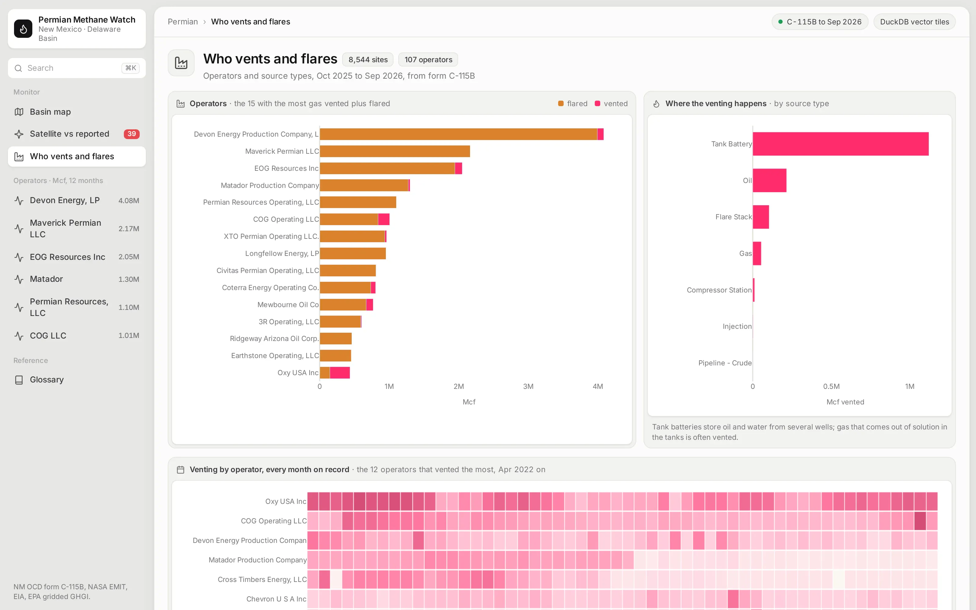
This page ranks operators by the gas they vented and flared over the last 12 months and shows which kinds of sites the venting comes from. Tank batteries, where oil and water from several wells are stored, stand out.
A heatmap of venting by operator and month shows who has been cutting back and who hasn't since monthly reporting began. A table under it lists every reporting site, and clicking a row opens it.
Open any site and see its history
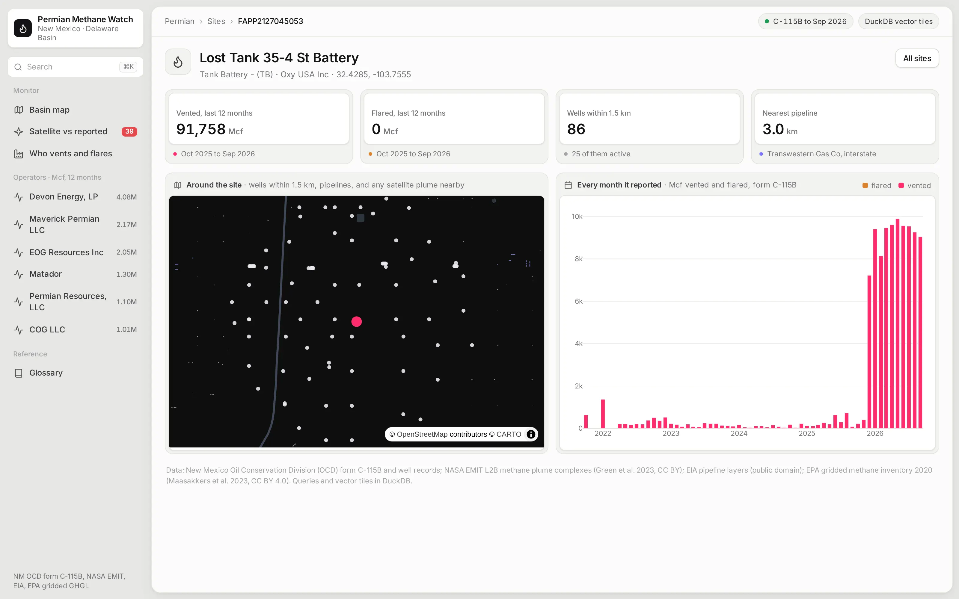
Every reporting well and facility has a page with each month it reported, split into vented and flared gas. A sudden change, like a site that vented almost nothing for years and then started venting every month, jumps out.
A zoomed map shows the wells within 1.5 km and the pipelines around it, and the app works out the distance to the nearest gas pipeline, which is often the first question when gas is being vented or flared instead of sold.
Ask the app from an AI agent
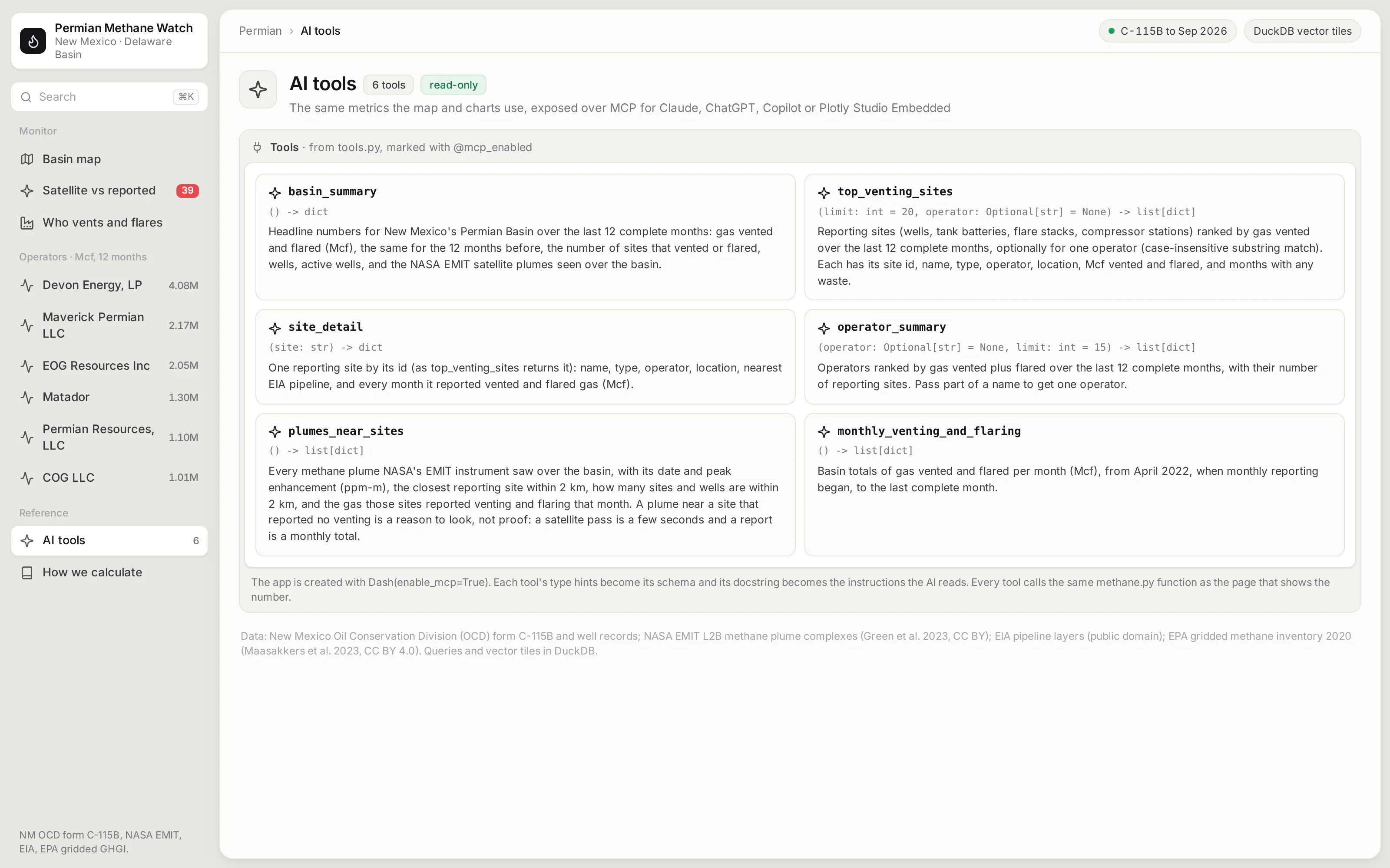
The app is also an MCP server. Six of its Python functions are marked with @mcp_enabled, so an AI agent connected to the app can ask which sites vented the most, how one operator compares, or which satellite plumes had venting reported nearby, and get the same numbers the map and charts show. Each tool's type hints become its schema, and its docstring becomes the instructions the agent reads:
from dash.mcp import mcp_enabled@mcp_enabled(expose_docstring=True)def top_venting_sites(limit: int = 20, operator: Optional[str] = None) -> list[dict]:"""Reporting sites (wells, tank batteries, flare stacks, compressor stations) ranked by gas vented overthe last 12 complete months, optionally for one operator (case-insensitive substring match)."""s = M.site_totals().sort("vented", descending=True)if operator:s = s.filter(pl.col("operator").str.to_lowercase().str.contains(operator.lower(), literal=True))return _records(s, min(limit, 200))
Ask it inside the app with Plotly Studio Embedded
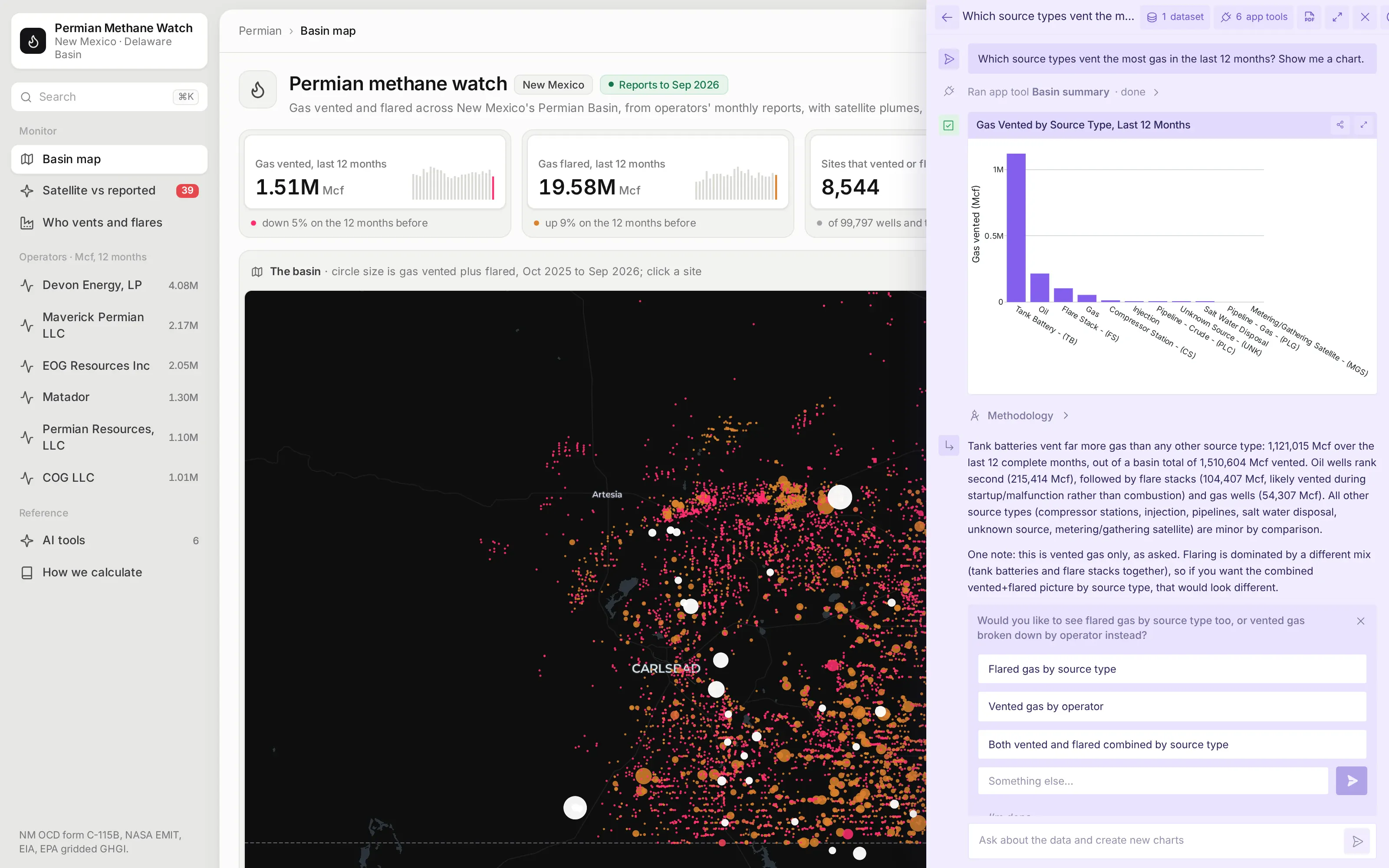
On Plotly Cloud you can switch on Plotly Studio Embedded, a chat panel that sits on top of the app and calls the same tools. Asked which source types vent the most gas in the last 12 months, it ran the app's basin_summary tool and drew the chart from what the tool returned, so its numbers match the app's own pages.
Studio Embedded is available on Plotly Cloud now and comes to Dash Enterprise in Q4 2026. Every answer has a Methodology link that shows the tool calls and code behind it.
See how every number is defined
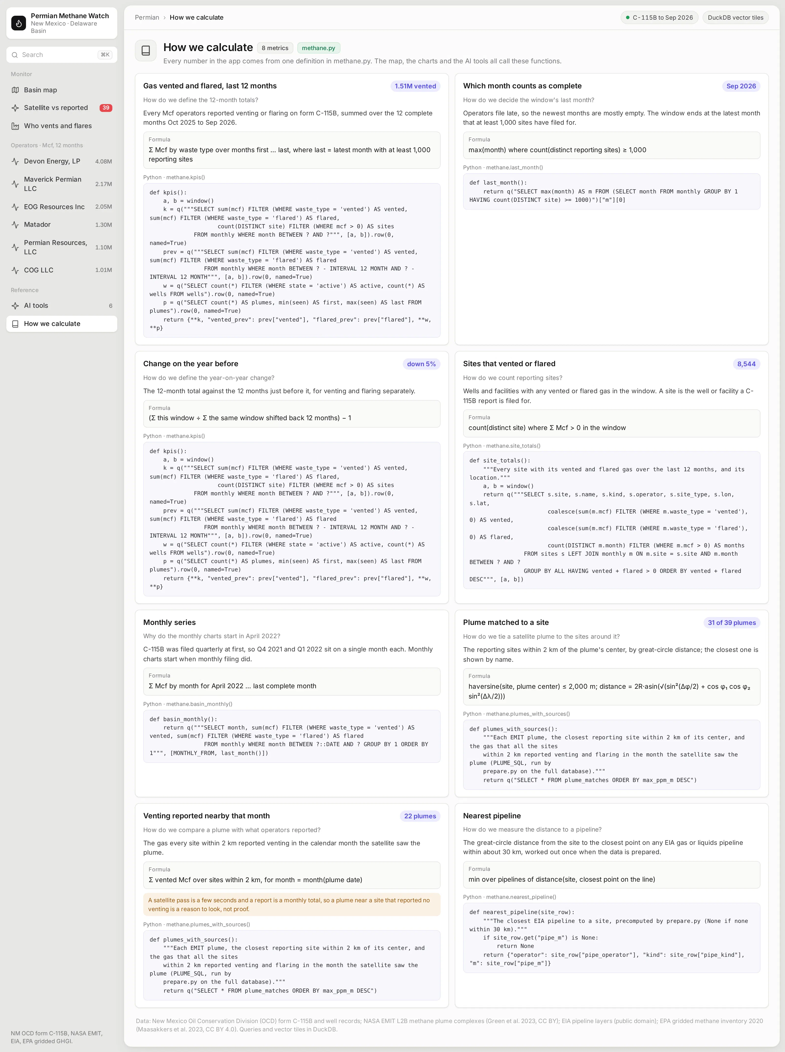
Which months count as complete, how a plume gets tied to the sites around it, and what "venting reported nearby" means are choices that change the numbers. This page writes each one down: the question, the definition in plain words, the formula, and the Python function that computes it.
Those functions are the app's semantic layer. The map, the charts, and the AI tools all call the same ones, so a number means the same thing wherever it shows up.
What else could you add?
The prompt is a starting point. These are the kinds of things teams usually ask for next, and each one is a sentence or two more in the prompt:
- Your own leak detection and repair (LDAR) survey results, aerial survey data, or continuous monitors on the same map
- Write-back, so a field team can log that a flagged site was checked and what they found
- Alerts when a site's venting jumps against its own history
- Your own production data, to show venting as a share of gas produced
- Other states or basins your company operates in, where the data's terms allow it
How is this different from Spotfire and other BI tools?
If you're comparing Spotfire alternatives or other BI tools, the main differences come down to five things:
- With AI, apps like this can be built quickly and cheaply by anyone, including the emissions engineers and analysts who know the data best.
- The apps are backed by code, which you can version control, manage, and update more easily than a fleet of point-and-click dashboards, especially when AI is making the changes.
- The apps can go much further than a traditional BI tool, with multiple pages, write-back to databases, custom simulations, AI chart building inside the app, MCP endpoints, and more.
- You have full control over the app: the look and feel, the controls, filters, and buttons, and every computation. You aren't fighting a tool to get what you want.
- The apps can connect to several data sources at once, and to the other systems your team already uses.
How long did it take to build?
About 40 minutes of agent time. Claude Code (with Claude Opus 5.5) spent about 24 minutes finding and downloading the public data and checking each source's license, and about 18 minutes building the app, running it, and fixing what looked wrong in its screenshots.
It checked the data before building on it. It confirmed from the state's own filing guide that volumes are reported in Mcf, and it found that the first two reports were quarterly totals, so the monthly charts start when monthly reporting began in April 2022.
The prompt
Paste this into Claude Code, Codex, Copilot, Cursor, or another coding agent, in an empty folder. Swap in your own data source and the features you need.
Build a Dash app that monitors methane venting and flaring across New Mexico's Permian Basin, with DuckDB for every query and for the map's vector tiles.
Data
- Download New Mexico OCD's C-115B venting and flaring reports, its well locations, and its facility locations from the state's public GIS services. Check the volume unit in OCD's filing guide before you label anything.
- Add EIA's US natural gas pipeline layer, NASA EMIT methane plumes from the US Greenhouse Gas Center, and EPA's gridded methane inventory. Check each source's license and leave out anything that isn't open for commercial use.
- Load everything into one DuckDB file, with geometry in web mercator so tiles are cheap to build.
Map
- Serve the wells, pipelines, and EPA grid as vector tiles from a Flask route on the Dash server, built with DuckDB's ST_AsMVT. Draw them on a dark Plotly map, with the reporting sites and plumes as clickable traces on top and a button for each layer.
Pages (each with its own URL, and the back button must work)
- Basin: KPI cards for gas vented and flared in the last 12 months with the change on the year before, the map, a monthly chart of vented and flared gas, and the sites that vented the most.
- Satellite vs reported: each EMIT plume with the sites within 2 km and what they reported that month, with a caveat that a plume near a site is a reason to look, not proof.
- Operators: who vents and flares the most, which kinds of sites it comes from, and a heatmap by operator and month.
- /site/<id>: its monthly history, a zoomed map with the wells around it, and the distance to the nearest pipeline.
- A How we calculate page that shows how every metric is defined: the question it answers, the definition, the formula, and the Python function behind it.
- Expose the metrics as read-only MCP tools with `@mcp_enabled`, and list them on an AI tools page.
Design
- A light gray page with an inset sidebar and white cards. Each card has a title and a short description, with the chart or table inset in a white panel. Inter everywhere. No chart toolbars.
Run it, screenshot every page at 1600x1000, and fix anything that overflows, looks empty or doesn't match the numbers before you stop.
How do I run it on Dash Enterprise or Plotly Cloud?
Dash Enterprise runs Dash apps inside your own infrastructure, behind your firewall and even air-gapped, with single sign-on and access control for each app.
This app needs nothing special. It's a Dash app with a requirements.txt, and your coding agent can deploy it through the Dash Enterprise or Plotly Cloud command line. The tile route is part of the same app, so there's no separate tile server to run.
Keep the DuckDB file on a persistent filesystem so the app doesn't rebuild it after a restart, and point the app at it with an environment variable such as METHANE_DB=/data/methane.duckdb.
If you'd rather not run any infrastructure, Plotly Cloud hosts the same app for you. We tested this one there.
Tips and tricks
These are things we like doing when we build apps like this one.
- Serve big map layers as vector tiles. A few thousand points are fine as a Plotly trace, but 100,000 wells aren't. Building tiles with DuckDB and serving them from the app keeps the browser fast without a separate tile server.
- Keep the things people click as traces. Plotly's map layers don't hover or click, so put the bulk context in tiles and the sites people act on in a trace on top.
- Make the agent check licenses, not just the data. Public doesn't always mean open for commercial use. The agent left out Texas Railroad Commission data and Carbon Mapper's plumes because of their non-commercial terms.
- Put the caveat next to the chart. When two data sources measure different things, like a satellite snapshot and a monthly report, say so on the page.
- Let plain Python functions be your semantic layer. The venting totals, the 12-month window, and the plume matching are short functions over DuckDB, and you can read them, test them, and change them, and so can the agent. Plain Python functions like these can become your semantic layer, one definition that every page, test, and agent uses.
- Wrap your Python functions in @mcp_enabled. Turn on enable_mcp=True in the Dash(...) call and mark the functions with @mcp_enabled, and chat agents like Claude, ChatGPT, or Copilot can call them over MCP and get the same numbers the app's pages show.
- Switch on Plotly Studio Embedded. The same tools power Plotly Studio Embedded, an AI chat inside the app that answers questions with charts and tables built from your functions. It's available now on Plotly Cloud (in beta) and is planned for Dash Enterprise in Q4 2026.
FAQ
See what Dash Enterprise and Plotly Cloud can do for your team
Our customers in energy, pharma, finance, and manufacturing are building apps like this one with coding agents and running them on Dash Enterprise behind their firewall or on Plotly Cloud. Request a demo and we'll show you how it works for your team.