Candlestick Charts - A Complete Guide

TL;DR

• A candlestick chart draws one candle per period (a day, an hour, a week). The body spans the open and the close, the wicks reach the high and the low, and the color says whether the period closed up or down.
• Candlestick charts are also known as Japanese candlestick charts and K-line charts, and are similar to OHLC charts and line charts.
• Use one for prices and other values with a meaningful open, high, low and close: stocks, futures, currencies, crypto, yields and power prices. It shows the range inside each period, which a line of closing prices hides.
• Use a line chart instead for long trends and for comparing several series, and OHLC bars when color would suggest good or bad news.
• Any coding agent can make one with Plotly in a minute. In Python it's go.Candlestick(x=..., open=..., high=..., low=..., close=...), plus rangebreaks to hide weekends.

What is a candlestick chart?

Candlestick charts look like this:

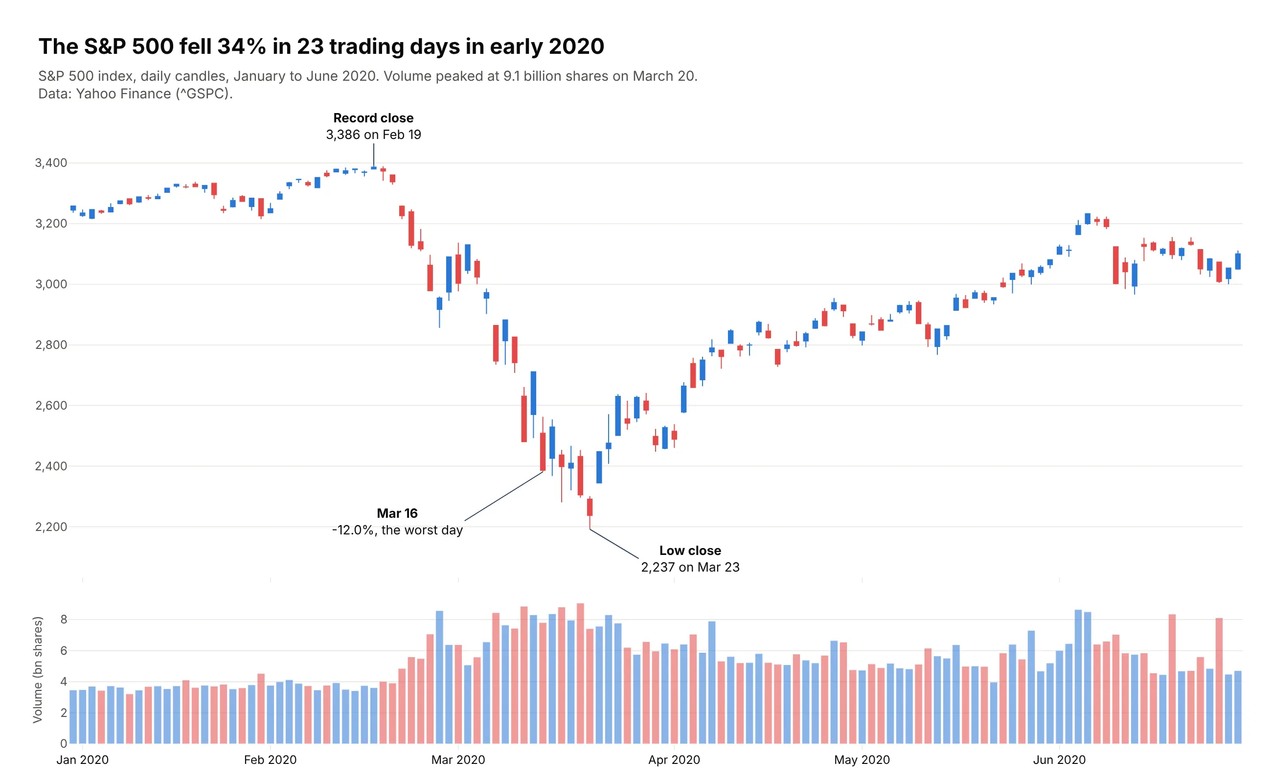
Data: Yahoo Finance (^GSPC).

How do you read a candlestick chart? In the example above, notice these things:

• Each candle is one trading day of the S&P 500, and its body runs from the day's opening level to its closing level. The body is blue when the index closed above where it opened and red when it closed below.
• The thin wicks above and below the body reach the day's high and low, so a long wick shows how far the index swung before it settled. In March the distance between a day's high and low averaged almost seven times what it was in January.
• Read the candles from left to right as one path. Most of the candles between the record close and the low close are red, and the first candle after the low close is a tall blue one that starts the climb back.
• The volume bars underneath share the same dates and colors, and they show trading was heaviest during the March sell-off, peaking on March 20, the last trading day before the low close.
• A candle's color only compares the close with that day's open. A few blue candles in late February and early March were days the index still ended lower than the day before, because it opened far below the previous close and won back only part of the gap.

It's often used for charts like these:

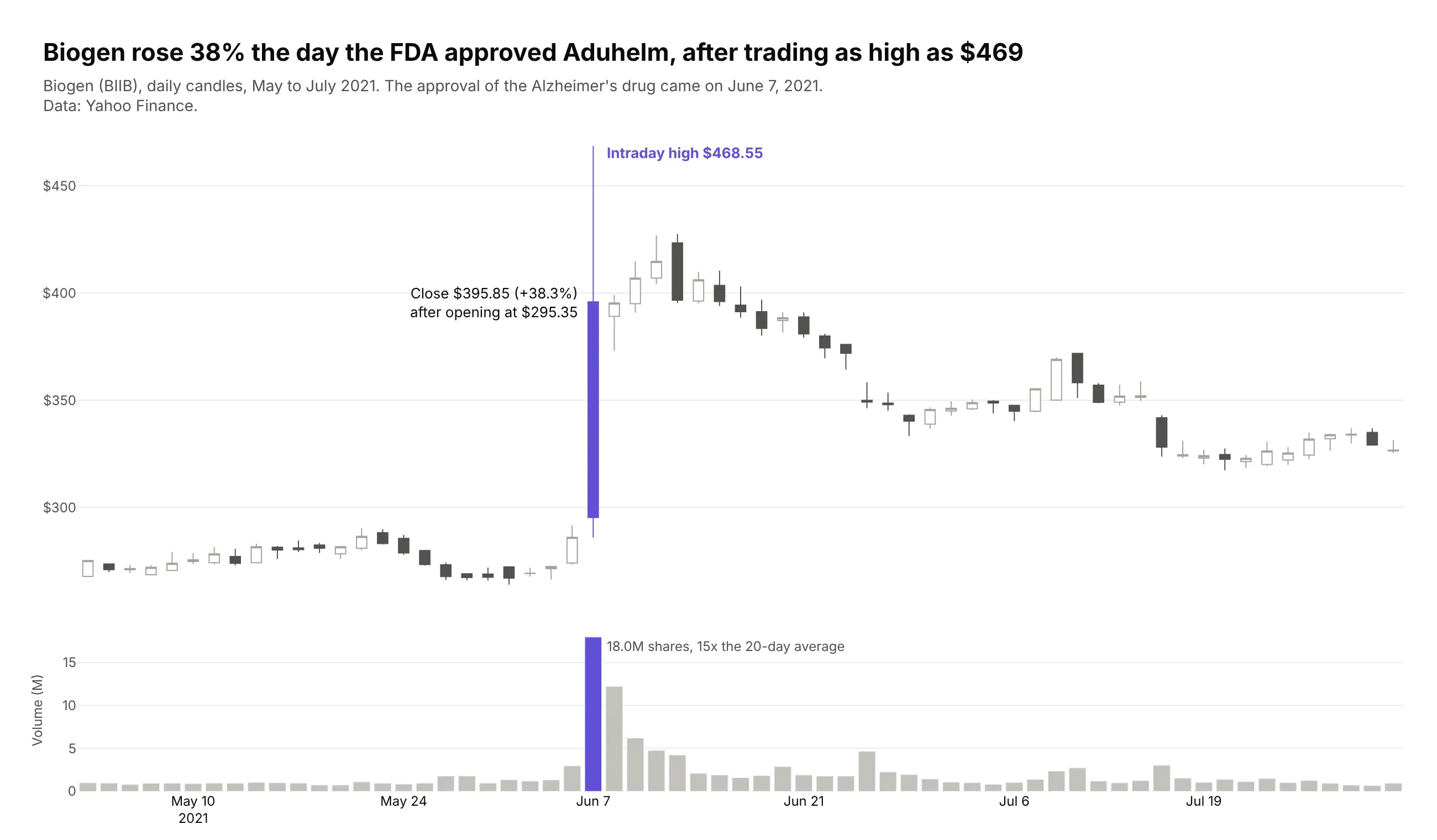
A stock on the day of big news. When the FDA approved Biogen's Alzheimer's drug Aduhelm on June 7, 2021, the stock traded as high as $468.55 and closed at $395.85, and the long upper wick is the part a line of closing prices loses. Data: Yahoo Finance (BIIB).

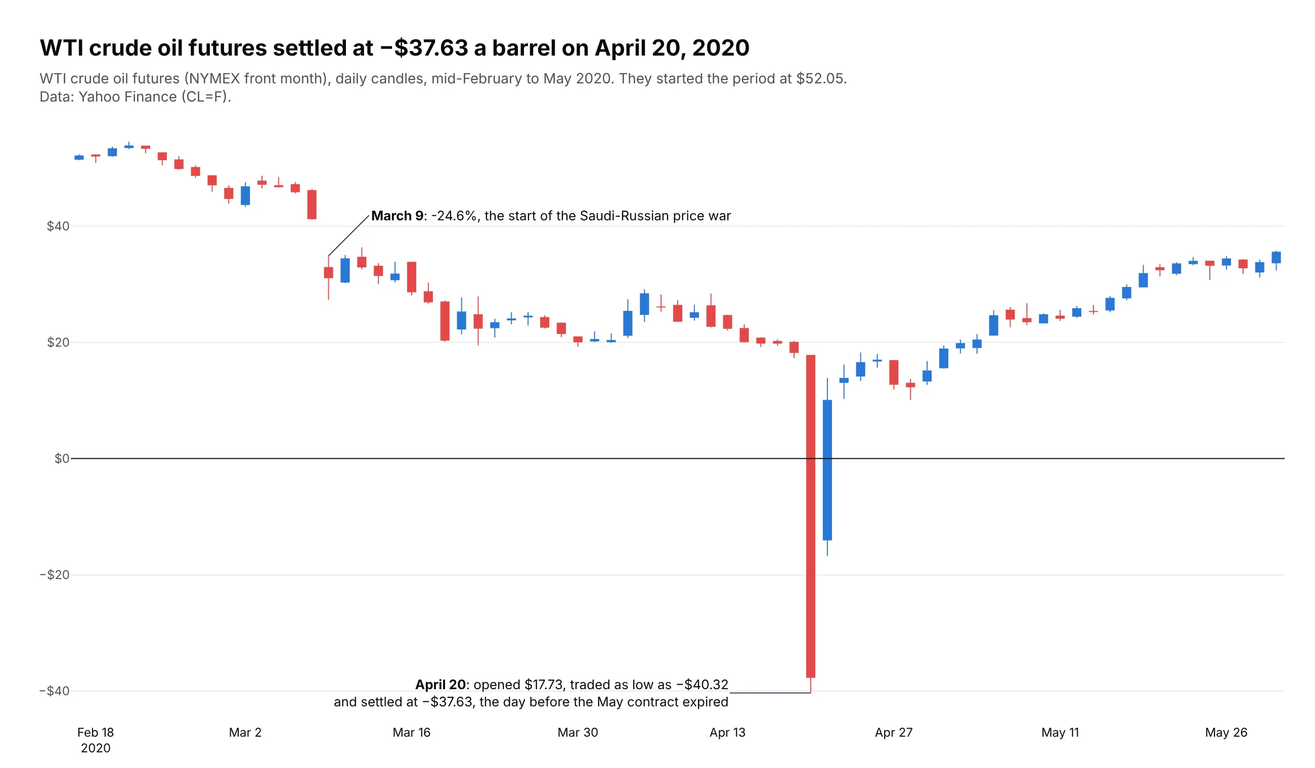
Commodity futures. On April 20, 2020, the day before the May contract expired, WTI crude opened at $17.73 a barrel, traded as low as -$40.32 and settled at -$37.63. Data: Yahoo Finance (CL=F).

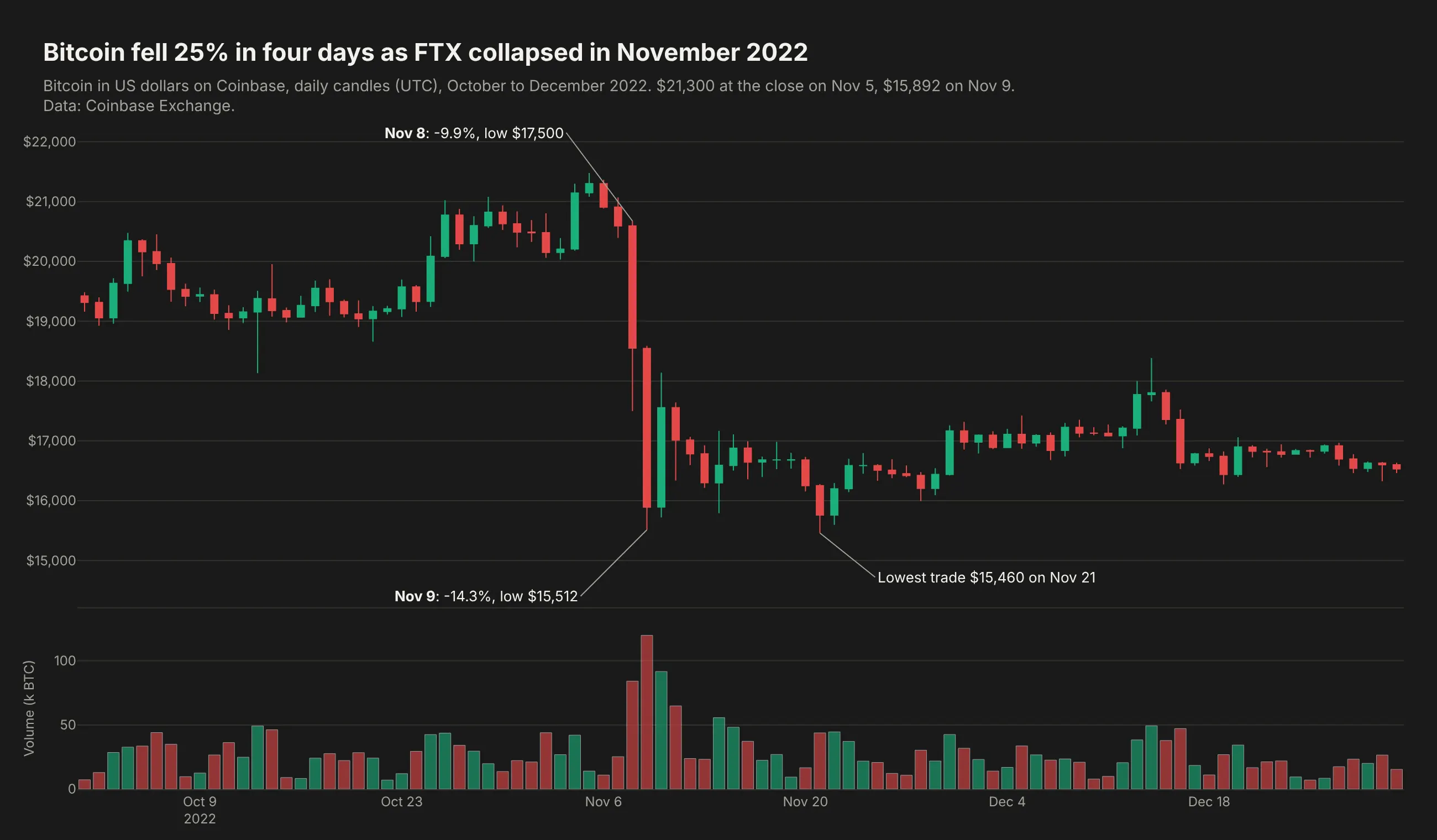
Crypto, which trades every day. Bitcoin fell 25% in four days as FTX collapsed, from $21,300 on November 5, 2022 to $15,892 on November 9, so this chart needs no rangebreaks for weekends. Data: Coinbase Exchange (BTC-USD).

A short history

Candlestick charts reached Western traders through Steve Nison's 1991 book Japanese Candlestick Charting Techniques (New York Institute of Finance), which traces them to Japanese rice trading and to the rice merchant Munehisa Homma in the 18th century. Before that, Western chartists drew OHLC bar charts, a vertical line from low to high with a tick on the left for the open and one on the right for the close, and Plotly has both as go.Candlestick and go.Ohlc. We haven't found price data from Homma's era in a form we can redraw honestly, so this guide doesn't recreate an original chart.

Alternatives to a candlestick chart

Here's the same volatility spike drawn six ways. Some are better for the question, some worse, some just different:

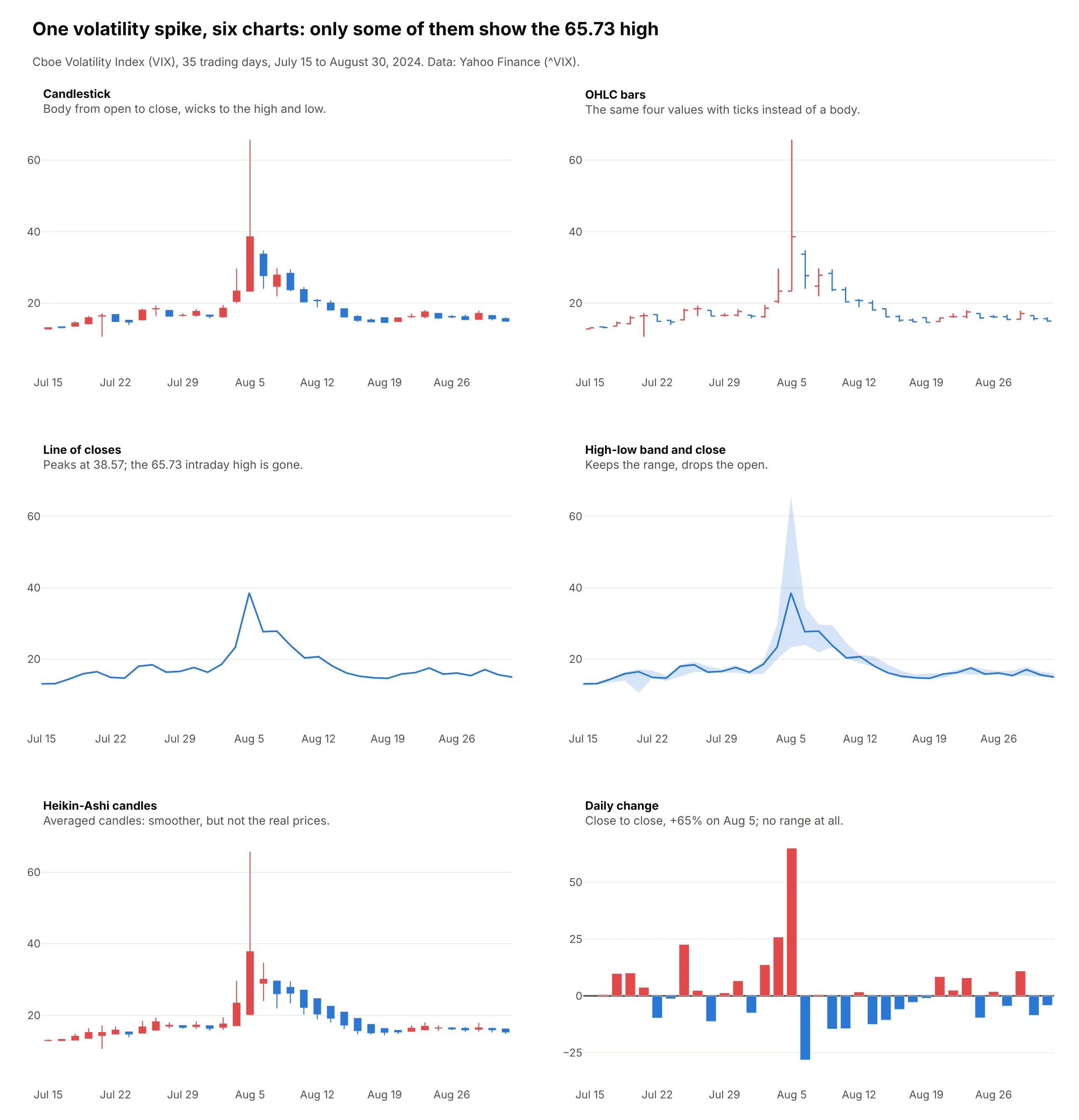
• OHLC bars (works too, and better for long series). The same four values with ticks instead of a body, so they use less ink with hundreds of bars and don't suggest that up is good when the series is a yield or a fear gauge (example 5 below).
• Line of closes (better for long trends and for comparing series). It's the clearest chart for years of data and for several assets indexed to 100, but it drops the range, so the VIX's 65.73 intraday high on August 5 disappears and the line peaks at the 38.57 close.
• High-low band with the close (works too, for readers who don't trade). A shaded band keeps the range and is easier to explain to a general audience. It leaves out the open.
• Heikin-Ashi candles (different). Each candle averages the period's prices with the previous candle, which smooths out the trend, but the bodies are no longer real opens and closes, so don't use them to report prices.
• Daily change bars (worse for the range, better for returns). Bars of the close-to-close change show that the VIX closed 65% higher on August 5, but nothing about how far it went during the day.

How to make a candlestick chart

With AI

ChatGPT, Claude Code, GitHub Copilot, Cursor and other AI tools are excellent at writing Plotly code. Name Plotly in the prompt, say what each candle should cover, and list the checks you want:

With Plotly Studio

Plotly Studio is a desktop app where you point an AI at a dataset and it builds charts and a Dash app around your questions. Ask for a candlestick chart the same way:

Show daily candlesticks of the S&P 500 for 2020 with volume underneath, hide weekends and holidays, label the worst day and add a dropdown to switch between daily, weekly and monthly candles.

Make a candlestick chart in Python or JavaScript

This is the code AI tools write under the hood. In Python, pass the four price columns to go.Candlestick and hide the weekends:

In JavaScript, plotly.js takes the same four arrays and a date for each candle:

For an OHLC chart in Python, swap go.Candlestick for go.Ohlc with the same four columns. The plotly.js version works as a JavaScript stock chart on any web page, and in React the Plot component of react-plotly.js takes the same trace and layout. To make weekly or monthly candles from daily data, resample with pandas before you plot: df.resample("W-FRI").agg(dict(open="first", high="max", low="min", close="last")).

Share it

Every Plotly chart has a Share chart button (the cloud icon in its toolbar) that uploads it to Plotly Cloud and gives you a link. Only you can see it until you change its visibility.

For a live app, put the chart in a Dash app and publish it with the Plotly Cloud CLI. Coding agents can run these commands for you:

If your data has to stay in your own cloud or data center, publish to Dash Enterprise instead.

Dos and don'ts

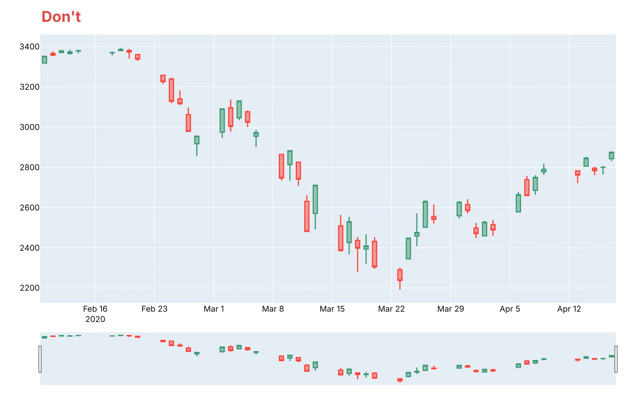
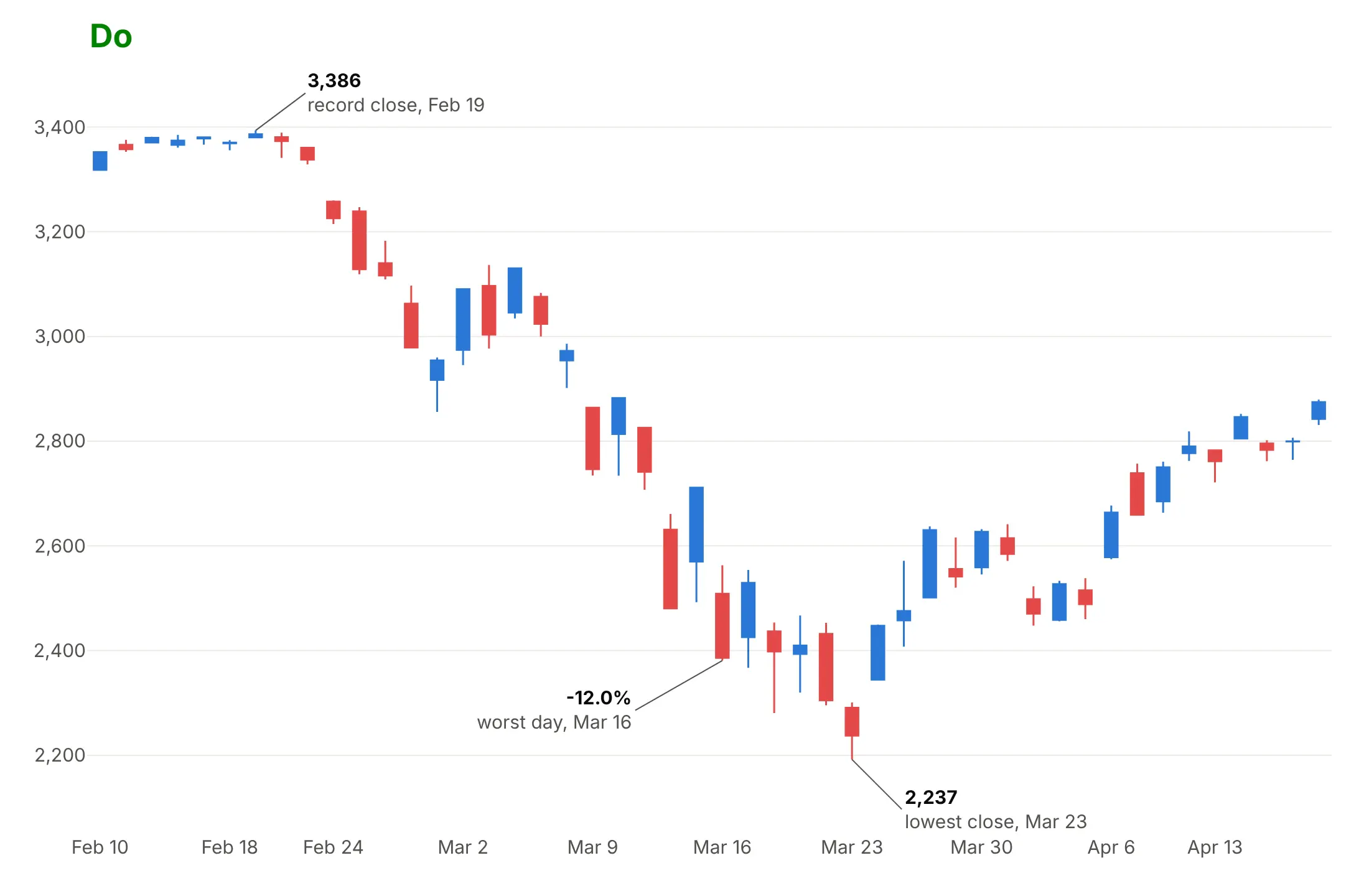
Plotly's default candlestick has a range slider under the x axis and leaves empty space for every weekend and holiday, because the x axis is a continuous date axis. For a published chart, most of the work is deciding what to leave out. Here is the S&P 500 from February 10 to April 17, 2020 both ways.

Don't publish the defaults, with gaps for every weekend and holiday, a range slider that repeats the chart, and no labels on the days that matter:

Do hide the closed days with rangebreaks, turn off the range slider and label the record close, the worst day and the lowest close:

Pick colors on purpose

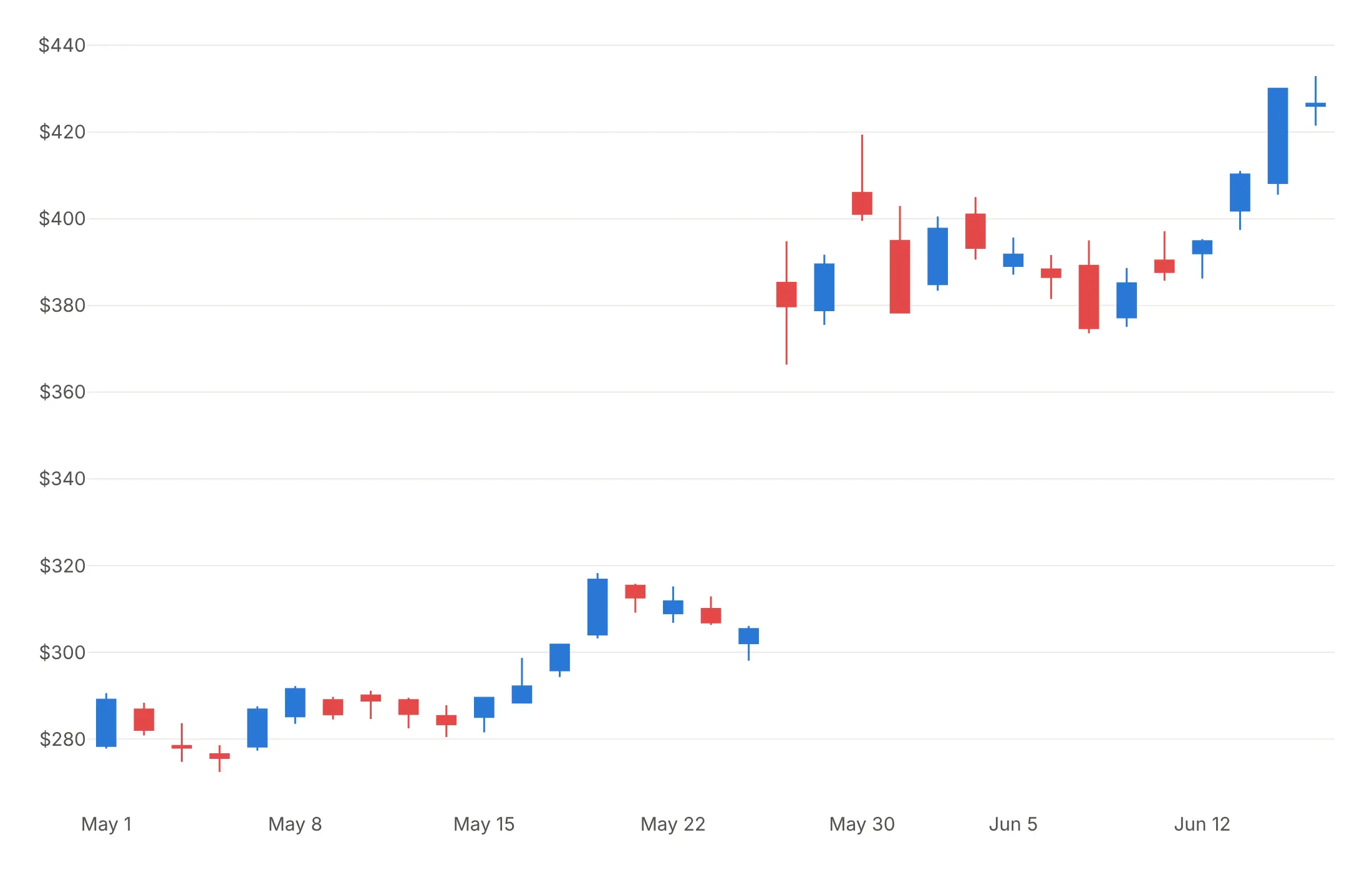
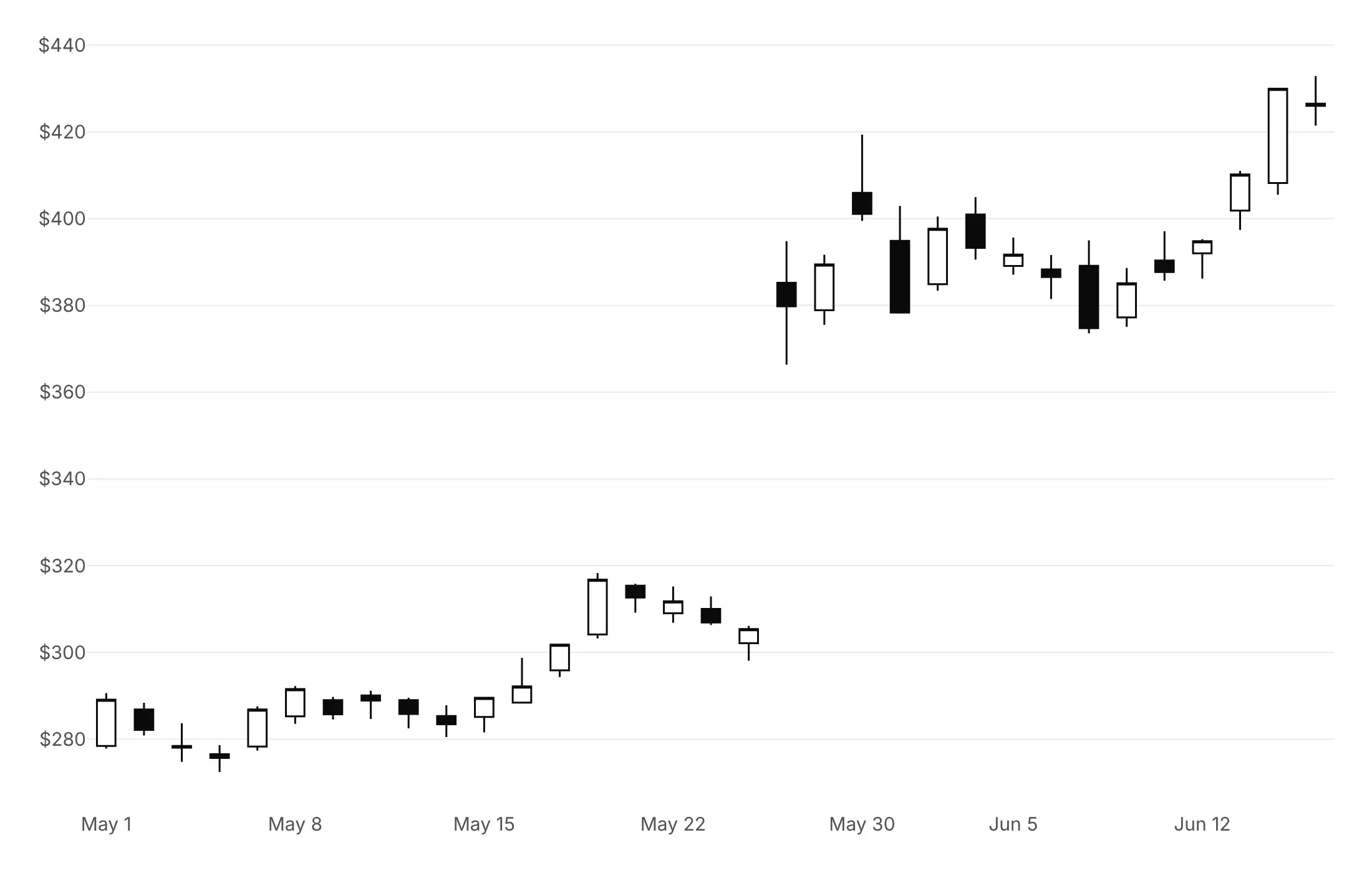
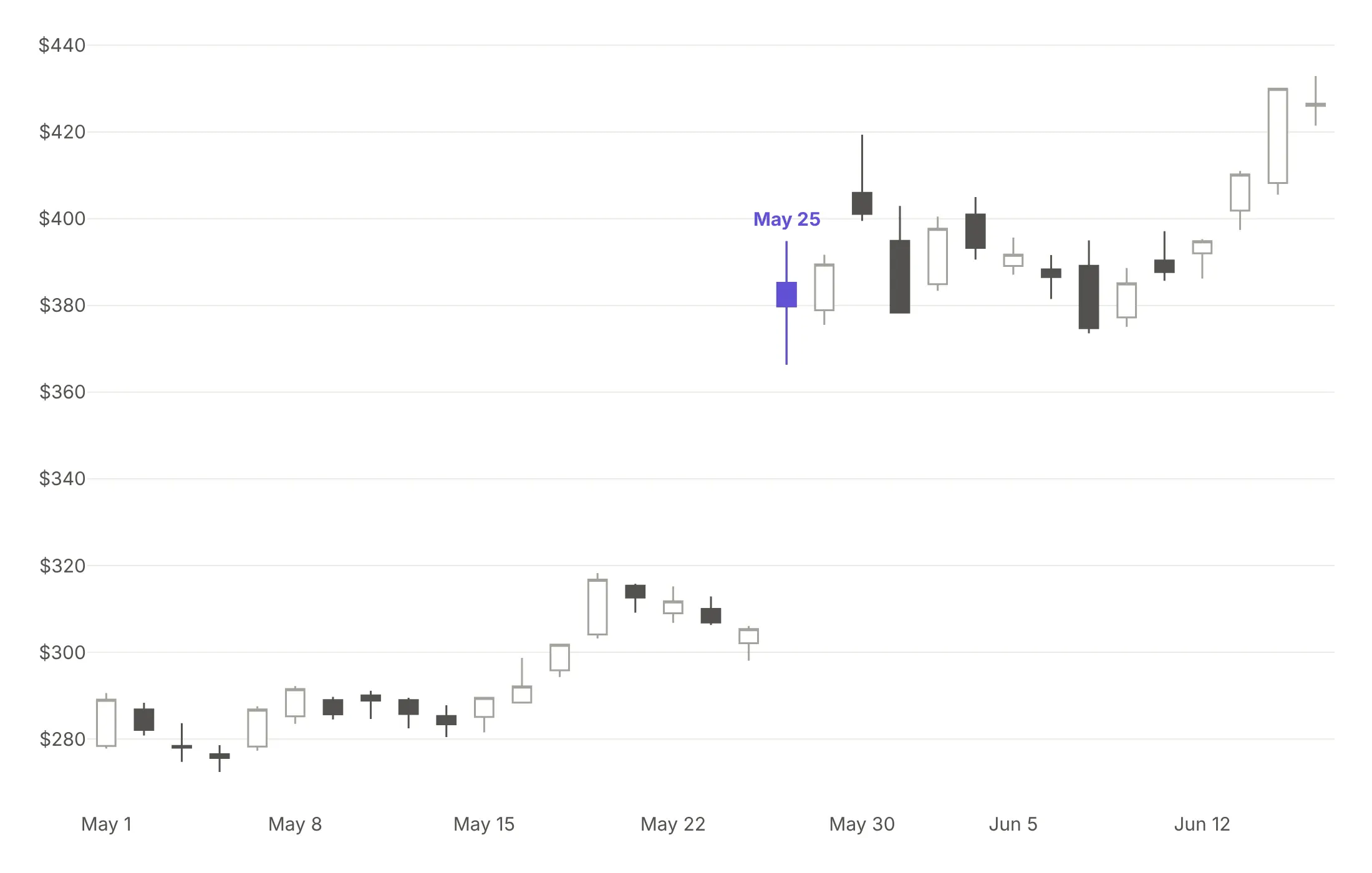
Here are four color schemes for the same Nvidia candles from May 1 to June 15, 2023, the weeks around its May 25 earnings gap.

Green and red. Familiar to traders, but hard to tell apart for readers with red-green color blindness.

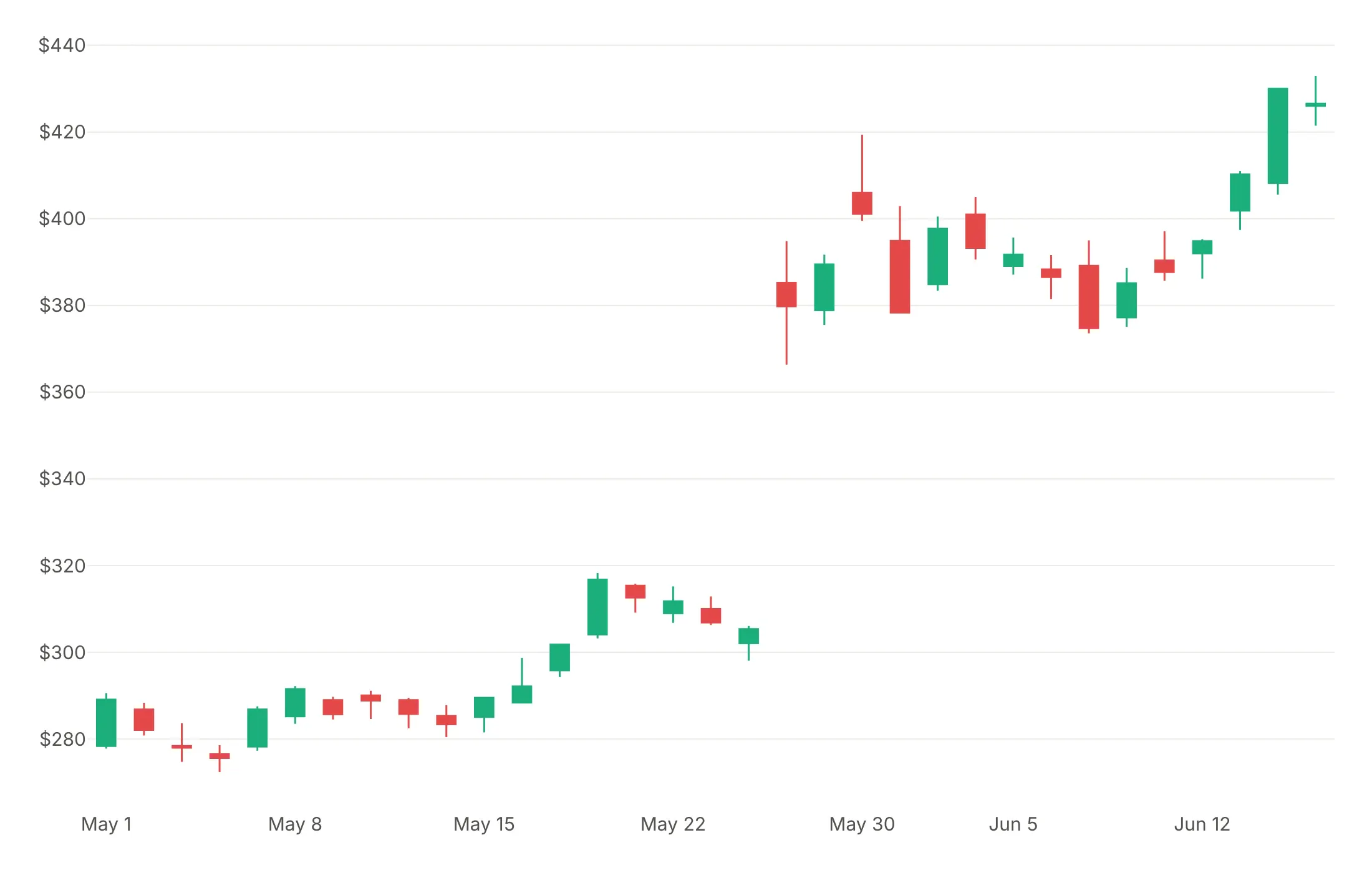
Blue and red. Still reads as up and down, works for most color vision, and it's what we use in this guide.

Hollow and filled in one color. Up candles are outlined and down candles are filled, which works in print and in grayscale.

Gray with one highlight. When one day is the story, draw everything else in gray and add that day as a second trace in one strong color.

Chinese and Korean platforms traditionally use red for up, so match your readers' convention. For a series where up is bad news, such as a volatility index or a bond yield, reverse the colors or use one color for both.

Checklist

Do

• Write a title that states what happened, with the number, and label the candles that matter.
• Hide non-trading time with rangebreaks: dict(bounds=["sat", "mon"]) for weekends, dict(values=holidays) for holidays and dict(bounds=[16, 9.5], pattern="hour") for nights in intraday data.
• Turn off the range slider in static images with xaxis_rangeslider_visible=False.
• Resample long histories to weekly or monthly candles.
• Put volume in a subplot with a shared x axis, colored like the candles.
• Use a log axis when prices span more than about 10x.
• Say in the subtitle whether prices are split-adjusted, which time zone the candles end in and what period each covers.

Don't

• Draw thousands of daily candles; about 250 on a 1,300-pixel-wide chart was the most we could fit before the bodies shrank to lines.
• Mix adjusted and unadjusted prices, or a stock split will look like a crash.
• Overlay many indicators. One or two, such as a moving average or a band, is plenty.
• Label a pattern as a "buy signal", because the chart can't support a prediction.

Options to customize

These are the go.Candlestick and go.Ohlc options that matter most. The full list is in the Plotly candlestick documentation and the OHLC documentation.

1. x, open, high, low, close: the period and its four values.
2. increasing.line.color, increasing.fillcolor: outline and body color of up candles; set the fill to white for hollow candles.
3. decreasing.line.color, decreasing.fillcolor: the same for down candles.
4. line.width: outline and wick width, thicker for a few candles and 1 px for many.
5. whiskerwidth: width of the wick caps from 0 to 1; use 0 for long series.
6. tickwidth (go.Ohlc only): length of the open and close ticks.
7. xperiod, xperiodalignment: the period each candle covers and where it sits in it, for weekly or monthly candles.
8. hoverlabel.split: shows the open, high, low and close as separate hover labels.
9. text, hovertext, yhoverformat: extra hover text and the number format.
10. xaxis.rangebreaks: hides weekends (bounds=["sat", "mon"]), hours (pattern="hour") or listed dates (values) in any market that isn't open around the clock.
11. xaxis.rangeslider.visible: the mini chart below the x axis, on by default; turn it off for static images.
12. xaxis.rangeselector: buttons such as 1M, 6M and YTD for interactive dashboards.
13. yaxis.type="log": a log price axis for prices that span more than about 10x.
14. make_subplots(shared_xaxes=True): panels that share the date axis, for volume or an indicator below the candles.

More candlestick examples

Eleven more candlestick and OHLC charts built from public price data, each with its source, the technique that makes it work and a prompt to rebuild it.

1. Nvidia's May 2023 earnings gap

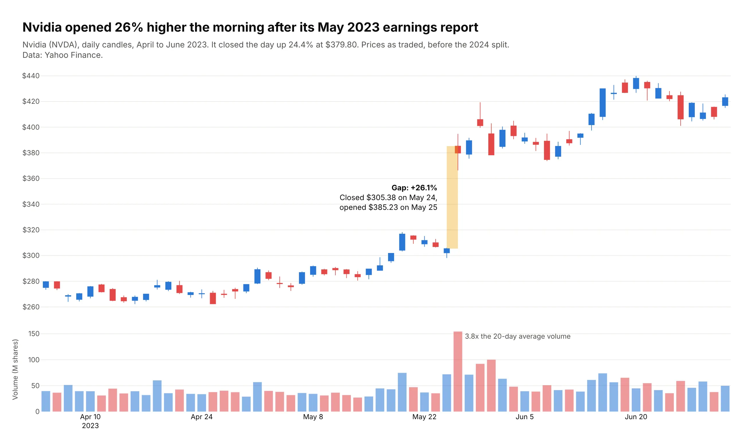
Nvidia closed at $305.38 on May 24, 2023, reported earnings after the bell and opened at $385.23 the next morning, a 26.1% gap. It closed the day up 24.4% at $379.80 on 3.8 times its 20-day average volume. Data: Yahoo Finance (NVDA), prices as traded.

Tip: shade the gap with fig.add_shape(type="rect") from the previous close to the new open.

2. Nvidia's 10-for-1 split, raw and adjusted

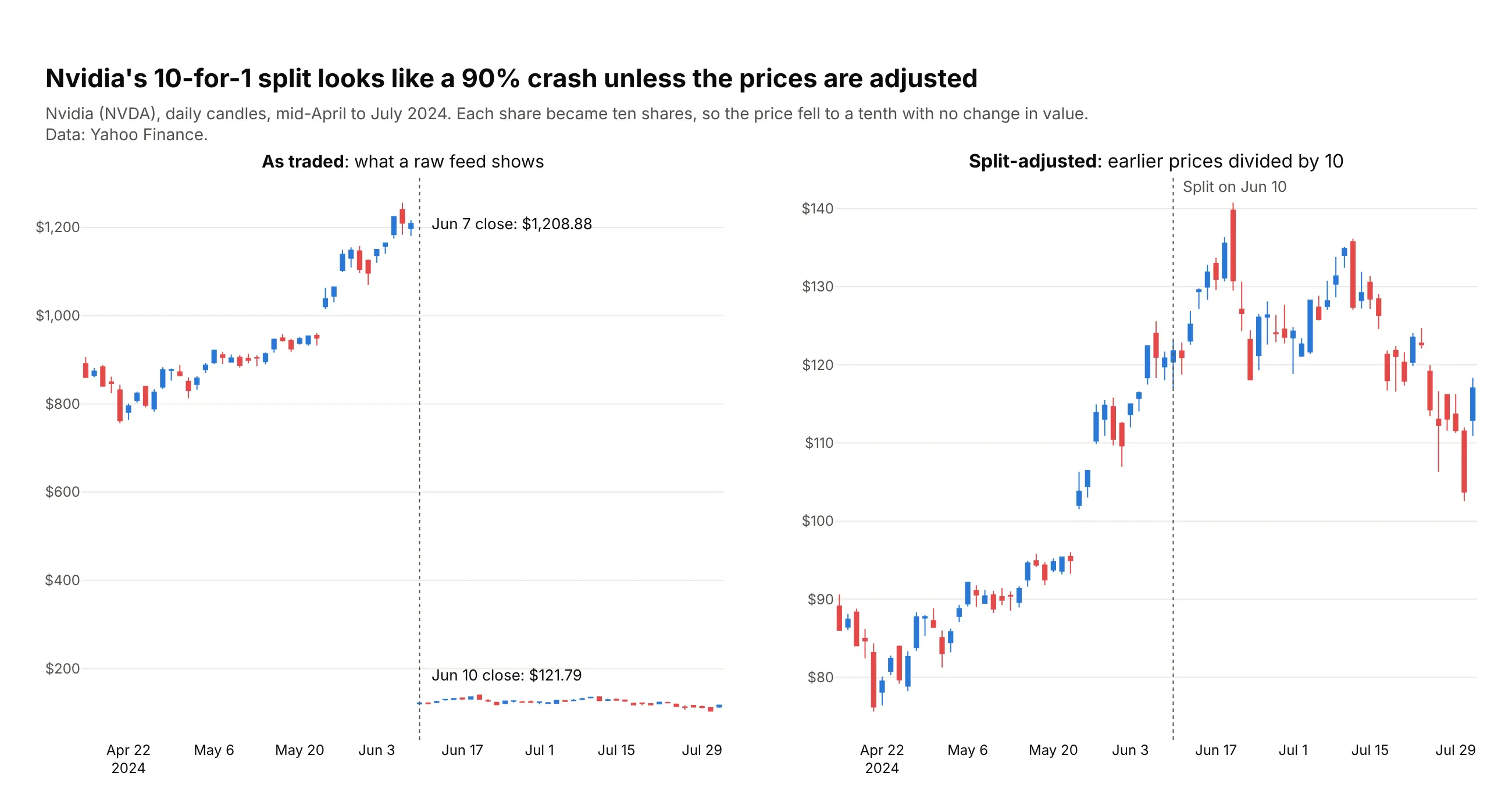
Nvidia closed at $1,208.88 on June 7, 2024 and at $121.79 on June 10, its first day after a 10-for-1 split. Raw prices show a 90% crash that never happened, which is why most feeds deliver split-adjusted prices. Data: Yahoo Finance (NVDA).

Tip: two subplots with independent y axes and a dotted add_vline on the split date in both.

3. The S&P 500 ETF, hour by hour, in the April 2025 tariff week

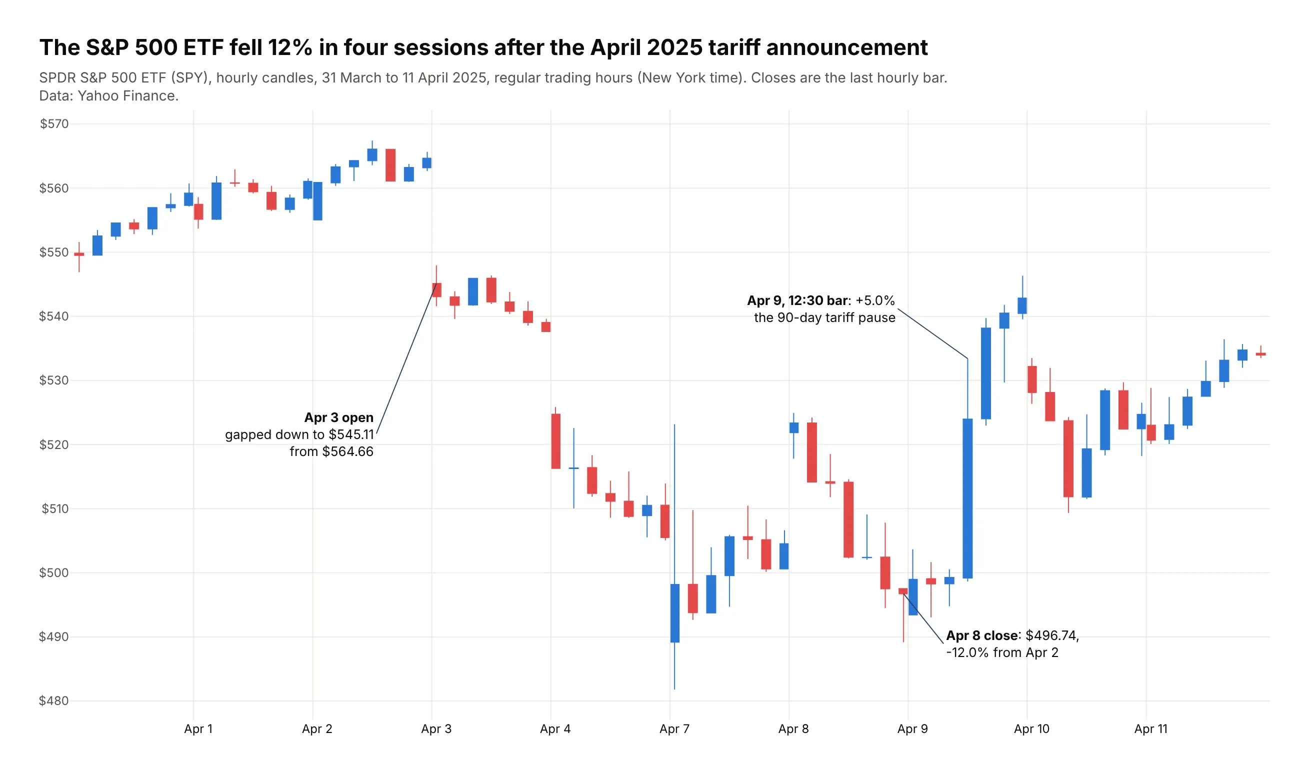
SPY fell 12% in four sessions after the tariff announcement on April 2, 2025, from $564.66 to $496.74 at the last hourly bar on April 8. On April 9 the 12:30 bar alone rose 5.0%, the hour the 90-day pause was announced. Data: Yahoo Finance (SPY), hourly bars.

Tip: rangebreaks=[dict(bounds=["sat", "mon"]), dict(bounds=[16, 9.5], pattern="hour")] removes nights and weekends.

4. The S&P 500's 2022 bear market with moving averages

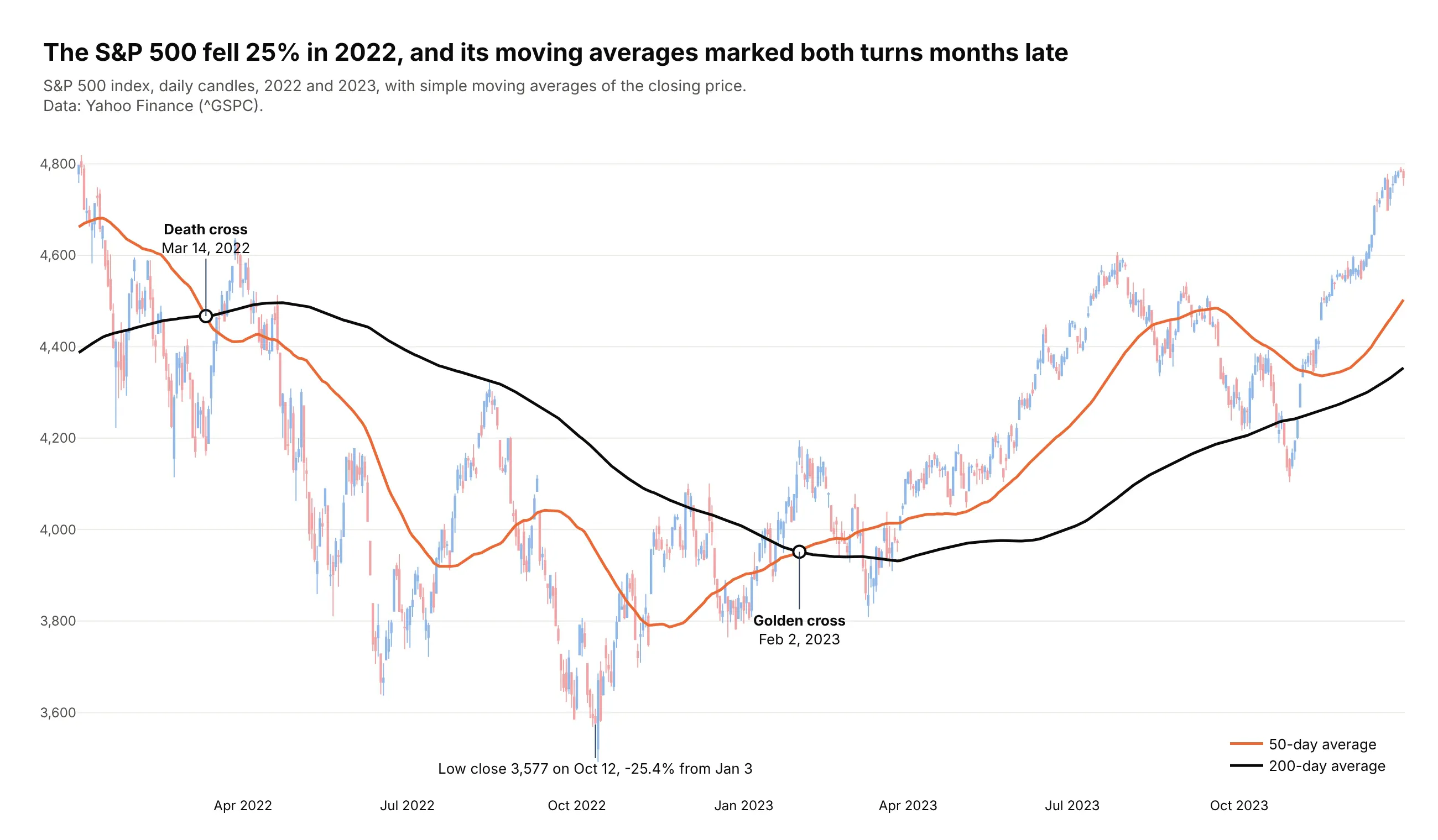
The S&P 500 fell 25.4% from January 3 to October 12, 2022. Its 50-day average crossed below the 200-day on March 14, 2022 and back above on February 2, 2023, months after each turn. Data: Yahoo Finance (^GSPC).

Tip: compute the averages on a year of earlier data, then slice, so the lines start on the first candle.

5. The VIX's August 2024 spike

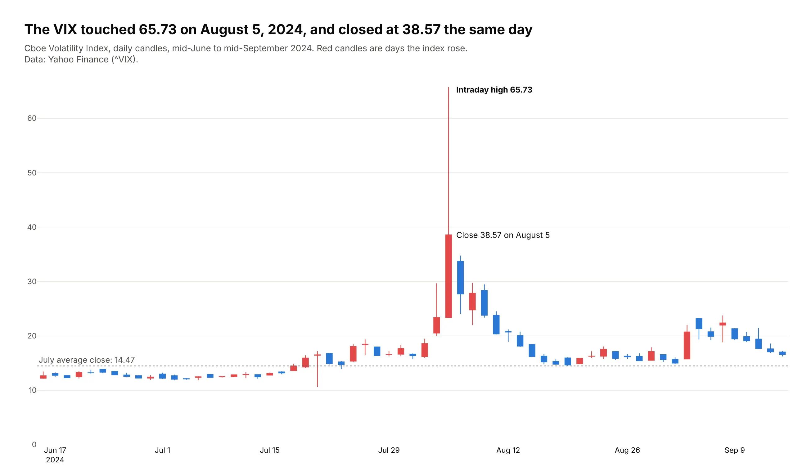
The VIX touched 65.73 on August 5, 2024 and closed at 38.57 the same day, against a July average of 14.47. The wick holds most of the move. Data: Yahoo Finance (^VIX).

Tip: reverse the colors for a fear gauge, so red means the index rose.

6. S&P 500 futures on election night 2024

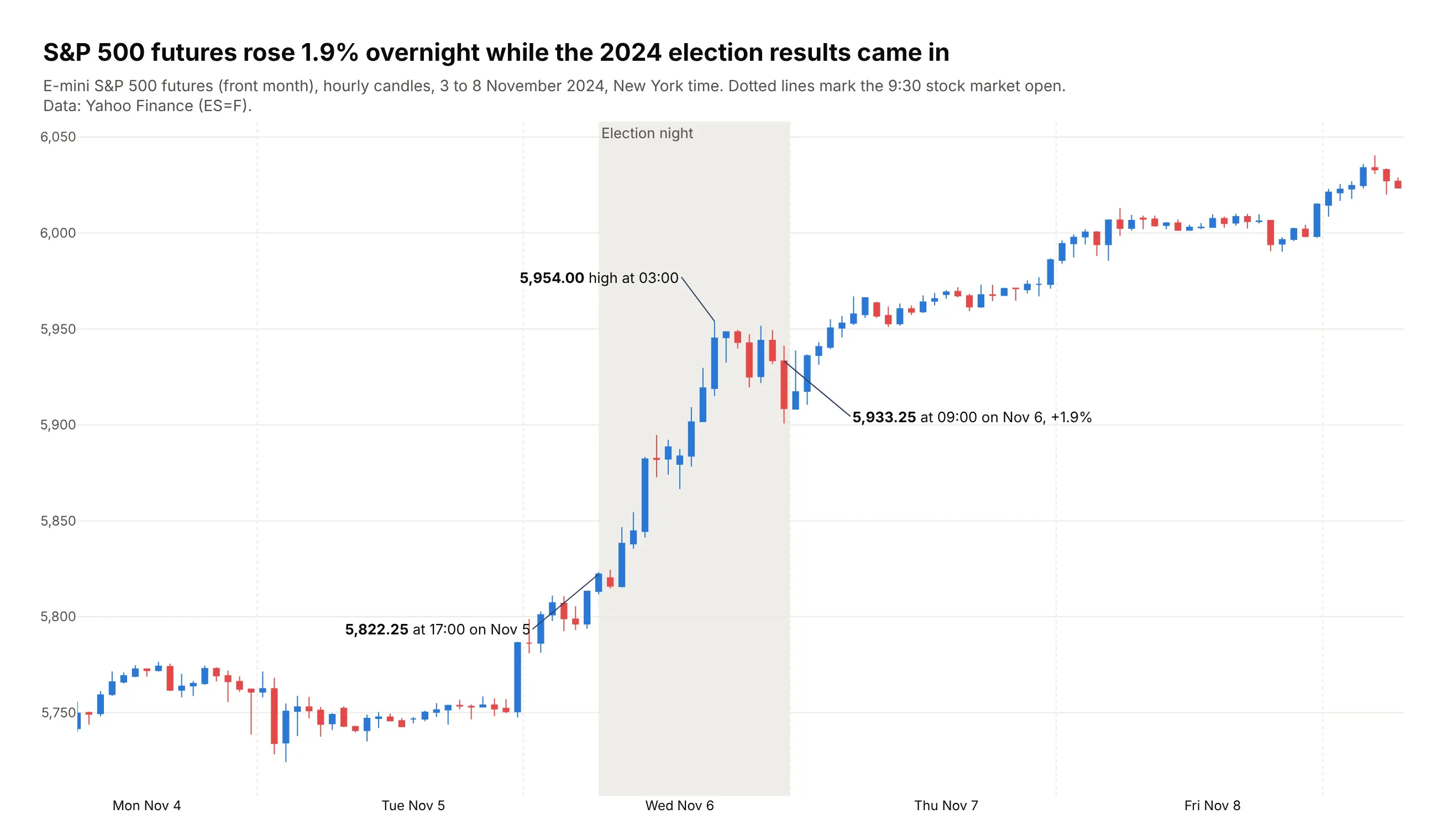
While the stock market was closed on election night, S&P 500 futures rose 1.9%, from 5,822.25 at 17:00 on November 5, 2024 to 5,933.25 at 09:00 the next morning. Data: Yahoo Finance (ES=F), hourly bars.

Tip: futures stop for one hour a day, so the rangebreak is dict(bounds=[17, 18], pattern="hour").

7. Henry Hub spot gas since 1997

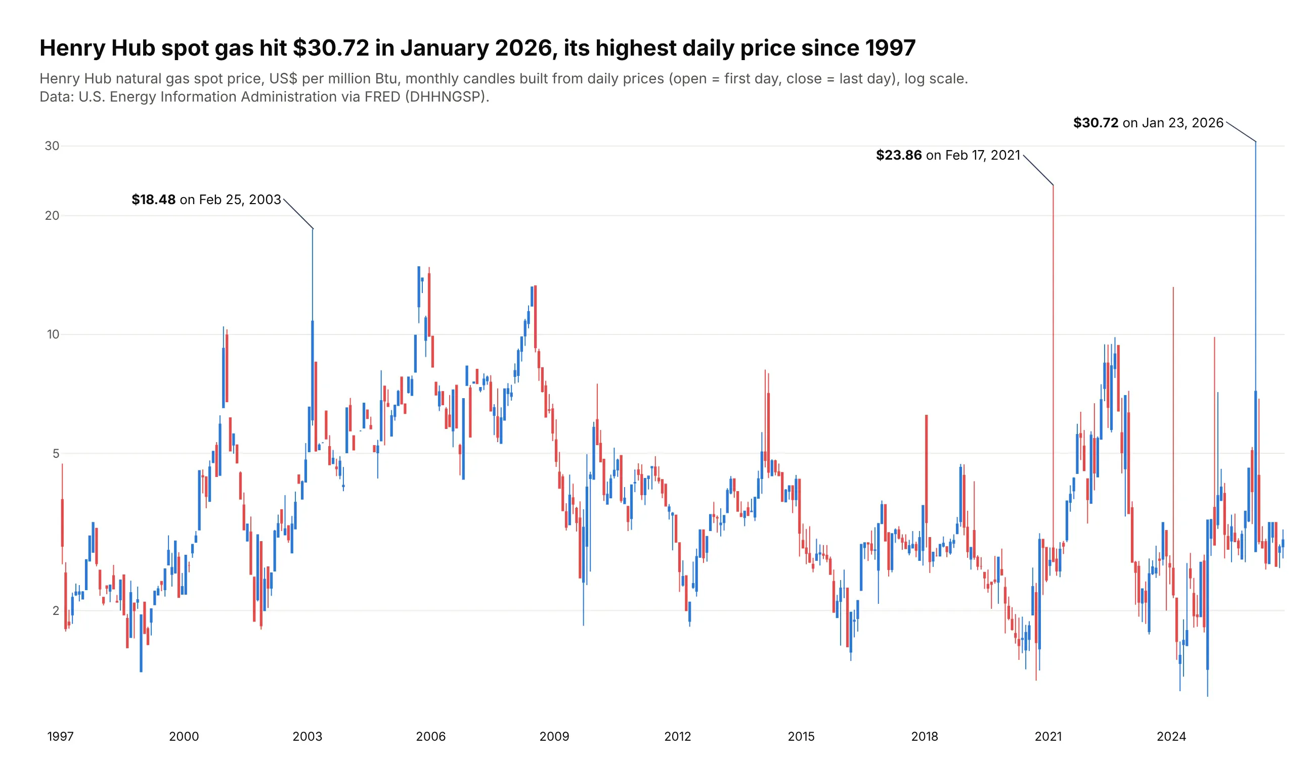
EIA publishes one Henry Hub spot price per day, so these monthly candles are built from 30 years of daily values. The highest day was $30.72 on January 23, 2026, above the $23.86 of Winter Storm Uri in February 2021. Data: EIA (RNGWHHD) via FRED.

Tip: any close-only series becomes candles with resample("MS").agg(["first", "max", "min", "last"]).

8. Houston power prices during Winter Storm Uri

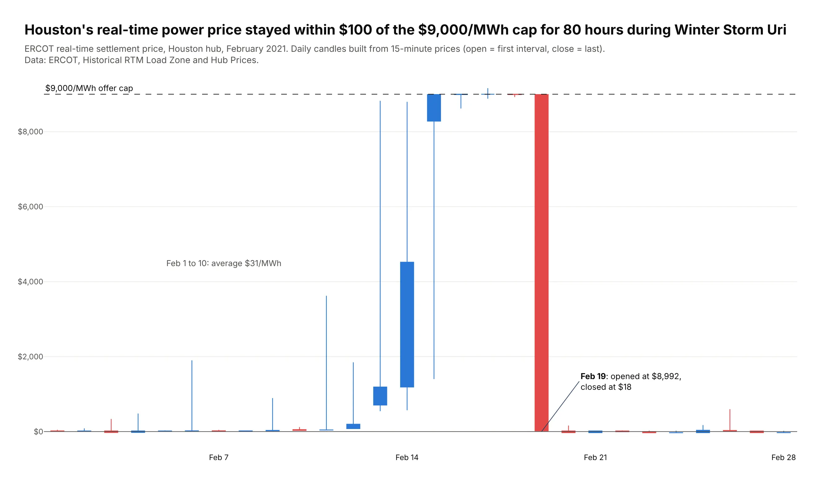
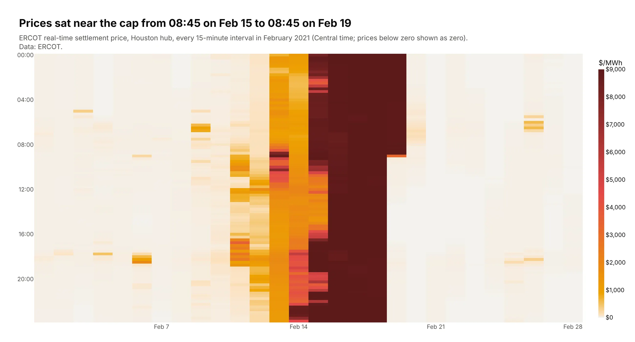
Houston's real-time power price stayed within $100 of ERCOT's $9,000/MWh cap for 80 hours during Winter Storm Uri, against a $31 average in the first ten days of February 2021. Data: ERCOT, Historical RTM Load Zone and Hub Prices.

Tip: daily candles from 15-minute data with resample("D"); open is the first interval and close the last.

Another way to see it: a heatmap of every 15-minute interval shows exactly when the price reached the cap and when it fell back.

9. The 10-year Treasury yield as OHLC bars

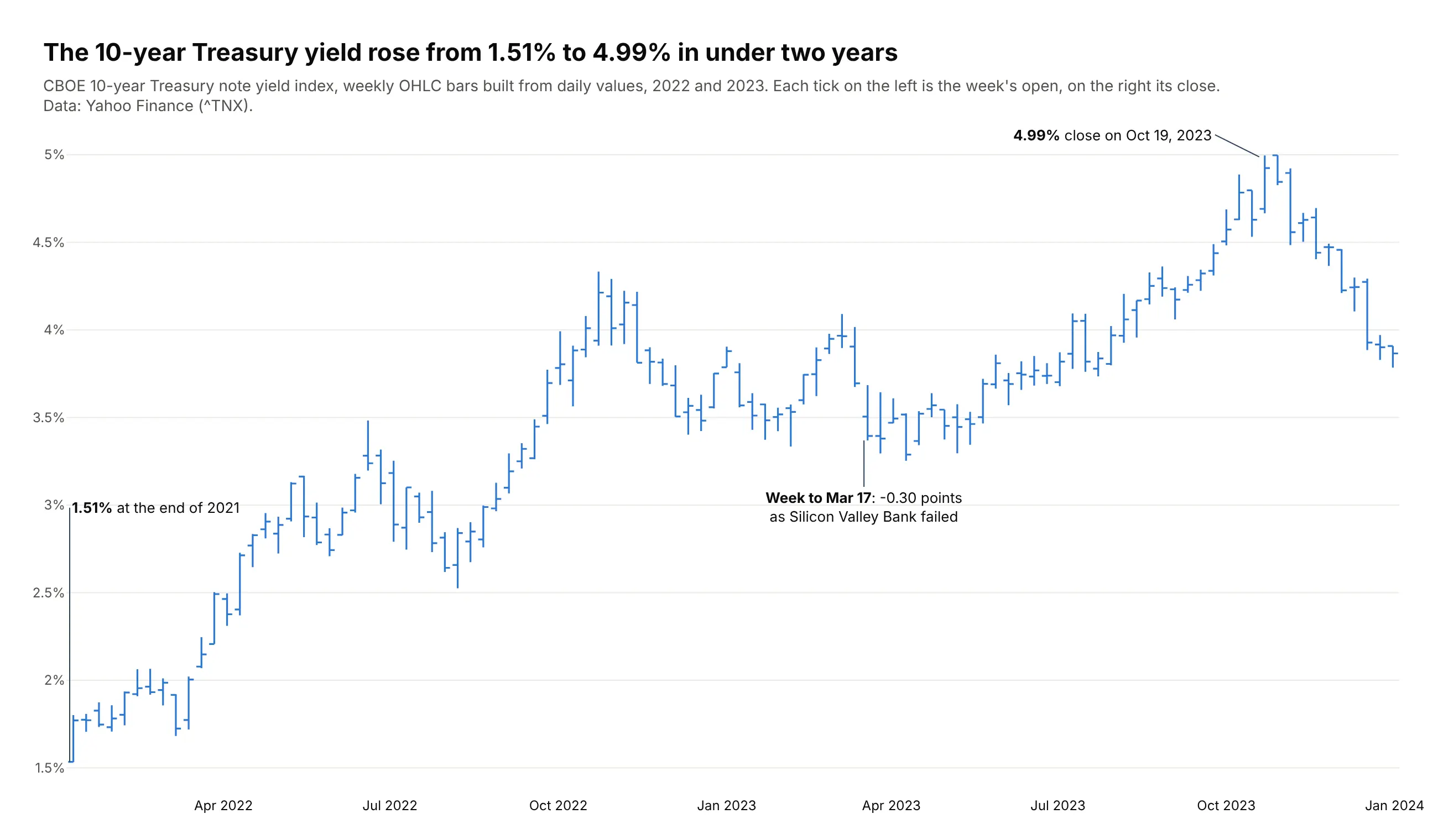
The 10-year Treasury yield rose from 1.51% at the end of 2021 to a 4.99% close on October 19, 2023. The largest weekly fall in March 2023, 0.30 points, came as Silicon Valley Bank failed. Data: Yahoo Finance (^TNX).

Tip: go.Ohlc with the same color for both directions, because a rising yield is neither good nor bad news by itself.

10. Bitcoin at three time frames

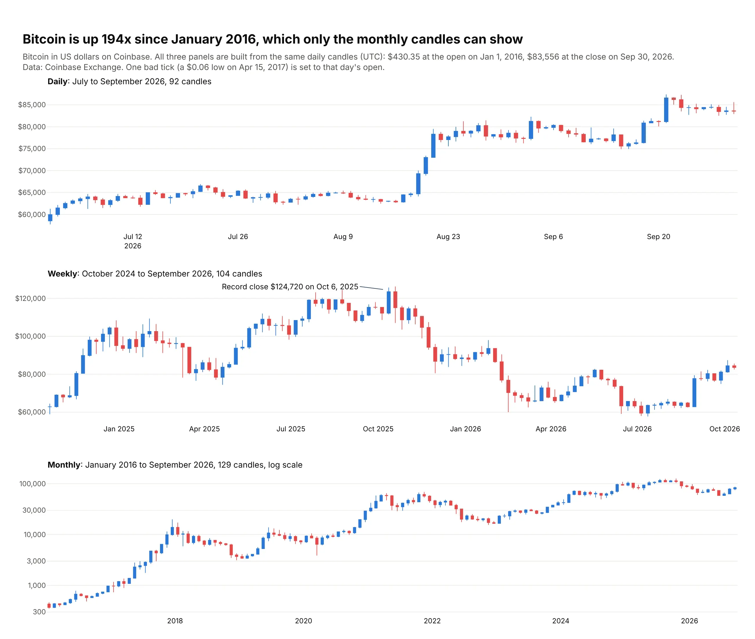
The same daily Coinbase prices give three different charts. Daily candles show the last quarter, weekly ones the 2025 record of $124,720, and only the monthly candles show the 194x rise since January 2016. Data: Coinbase Exchange (BTC-USD).

Tip: check for bad ticks before you resample; one $0.06 low in April 2017 would stretch a monthly candle to the bottom of the log axis.

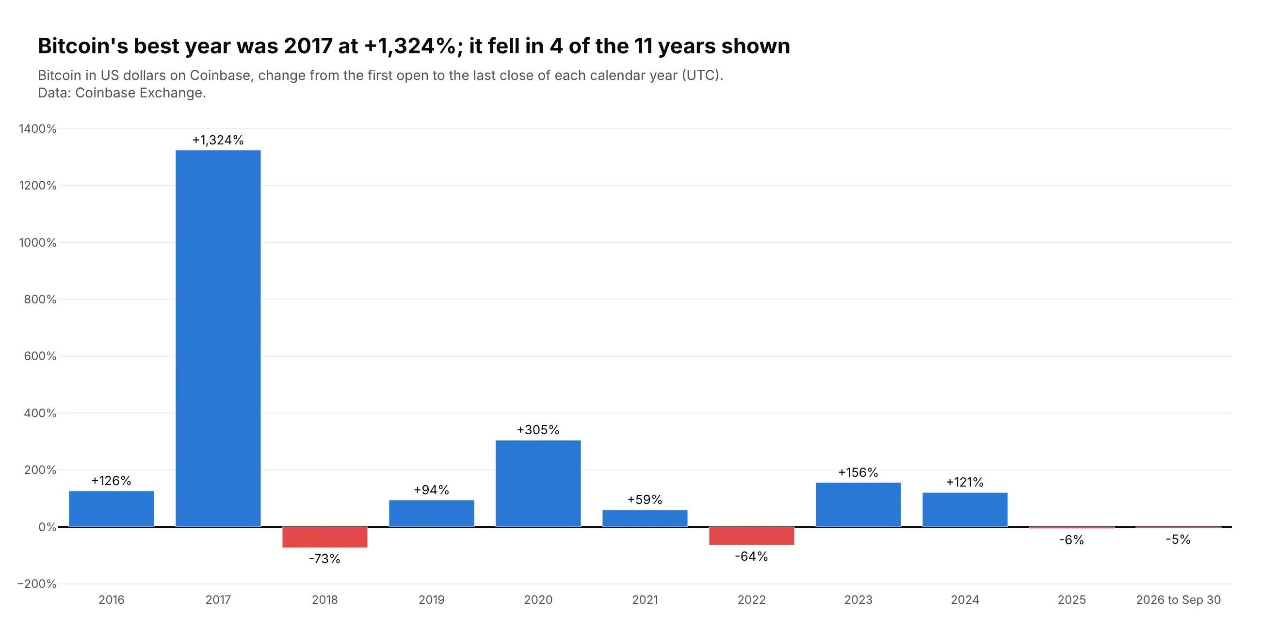
Another way to see it: a bar chart of each calendar year's return gives the same history in 11 bars.

11. The euro's April 2025 jump against the dollar

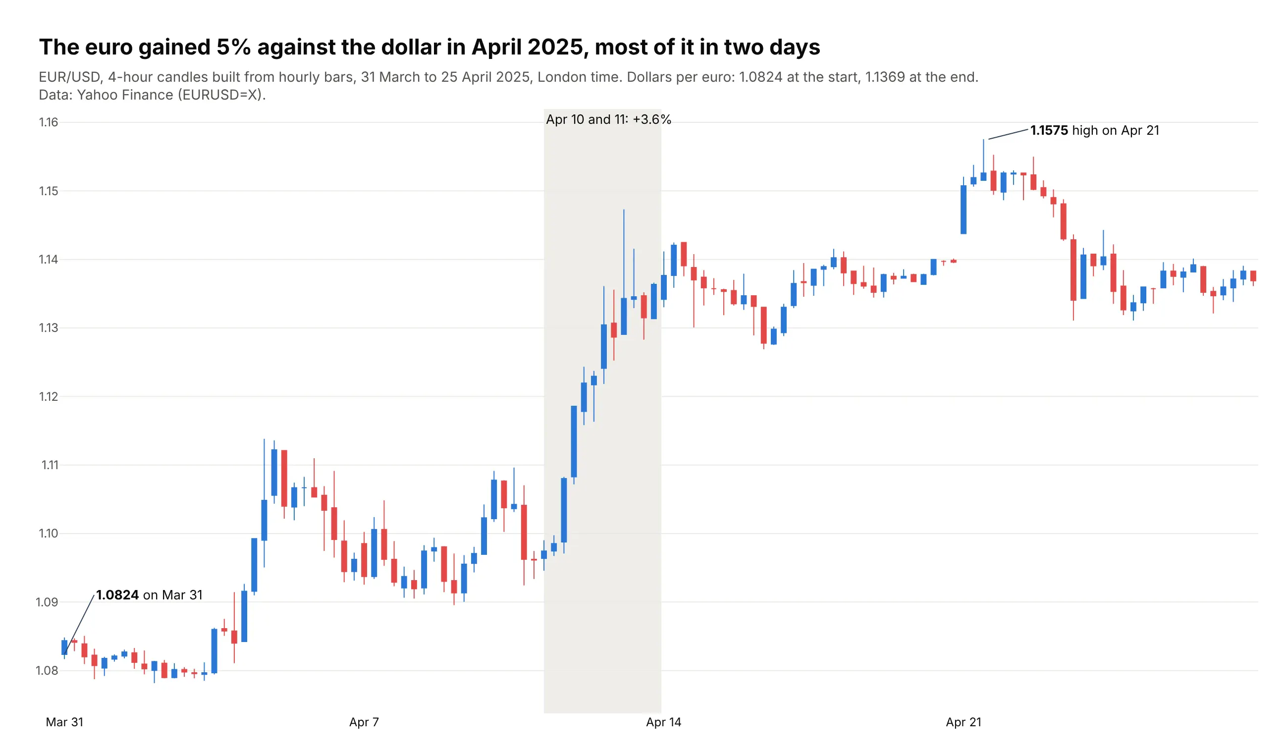
Currency pairs are one of the classic uses of candlestick charts, along with stocks and futures. The euro rose 5.0% against the dollar from March 31 to April 25, 2025, and it gained 3.6% on April 10 and 11 alone. Data: Yahoo Finance (EURUSD=X).

Tip: build the candles from hourly bars with resample("4h"), because Yahoo's daily FX bars report the open equal to the close; six candles a day show when the move happened.