Chris Parmer

October 27, 2026

UpSet Plots - A Complete Guide (with 10 Examples)

TL;DR

An UpSet plot shows how sets overlap: one bar per combination of sets, a dot matrix underneath that says which sets each bar is, and the size of each set on the side.
It replaces the Venn diagram once you have more than three sets. Six sets have 63 possible combinations, which a Venn diagram can't draw readably and an UpSet plot lists as columns.
Sort the bars by size to find the common combinations, or by degree (one set, two sets, three...) to read them in order, and add a box plot per bar to show a distribution.
You can make an UpSet plot with Plotly from go.Bar and go.Scatter traces in make_subplots. Any coding agent can write it, and the make_upset() helper below does it in about 80 lines.

What is an UpSet plot?

UpSet plots look like this:

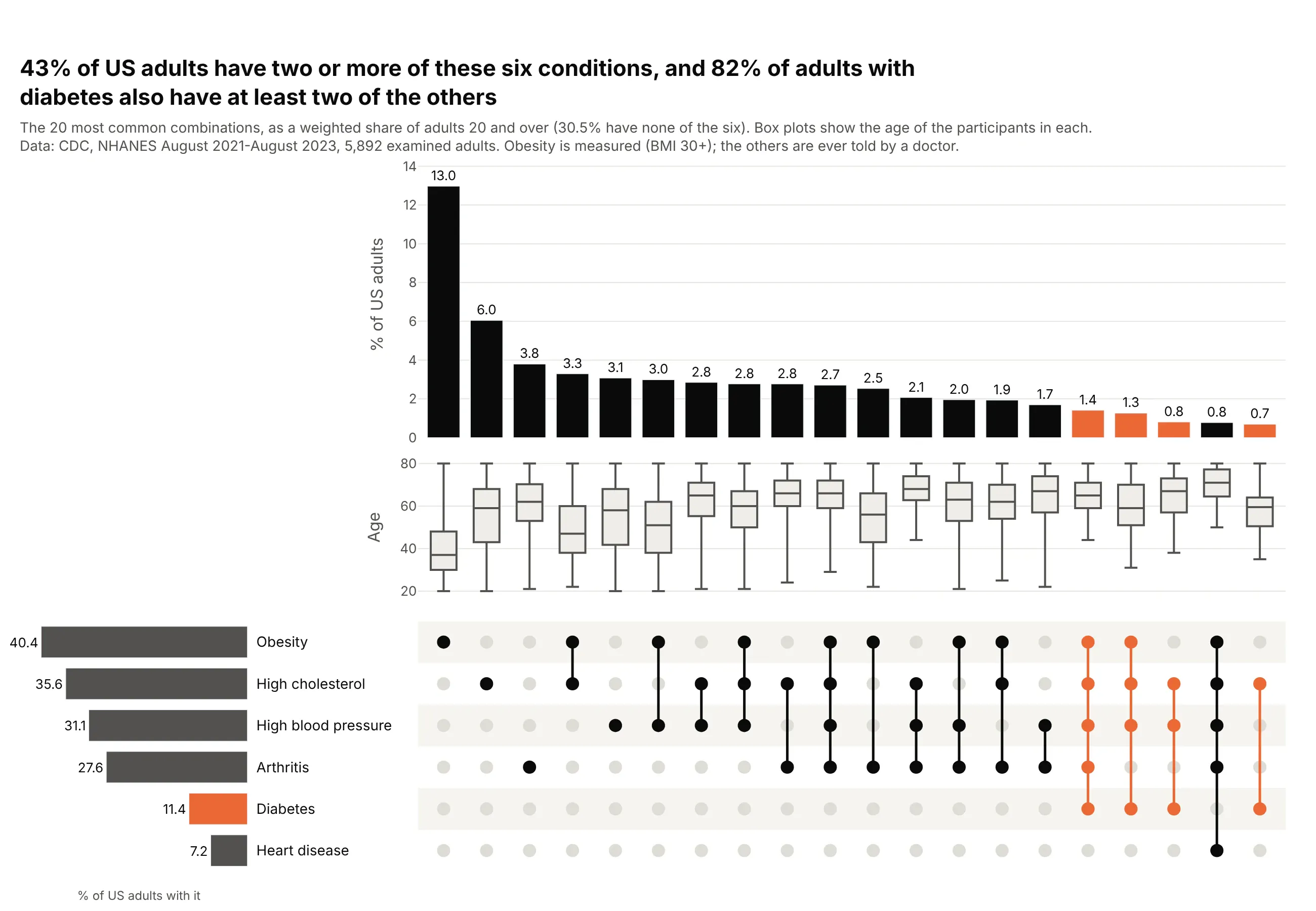
UpSet plot of six chronic conditions in US adults from NHANES 2021-2023, with 20 bars sorted by size. Obesity alone is the largest combination at 13.0% of adults, then high cholesterol alone at 6.0%. Combinations that include diabetes are orange, a row of box plots shows the age in each combination, and set bars on the left show obesity at 40.4% and heart disease at 7.2%

Data: CDC, NHANES August 2021-August 2023.

How do you read an UpSet plot? In the example above, notice these things:

Each column is one exact combination of conditions. The dark dots in the matrix say which conditions it includes, joined by a line when there is more than one, and the bar above is the share of US adults who have exactly those conditions and none of the others.
The columns are sorted from largest to smallest on a shared baseline, so the most common combinations come first and any two bars can be compared by height. Obesity alone is the tallest bar at 13.0% of adults, followed by high cholesterol alone.
Orange marks the columns that include diabetes, and they sit at the right end because each of them is small. Most of them join diabetes with two or more other conditions, which is the pattern the title points to.
The row of box plots shows the age of the people in each column. People with obesity alone have a median age of 37, and the boxes move up toward the 60s as more conditions join in.
The bars on the left are each condition's total, counting everyone who has it whatever else they have. Obesity's bar there is much longer than its own column because most adults with obesity also have another condition, so read totals on the left and overlaps in the columns.

It's often used for charts like these:

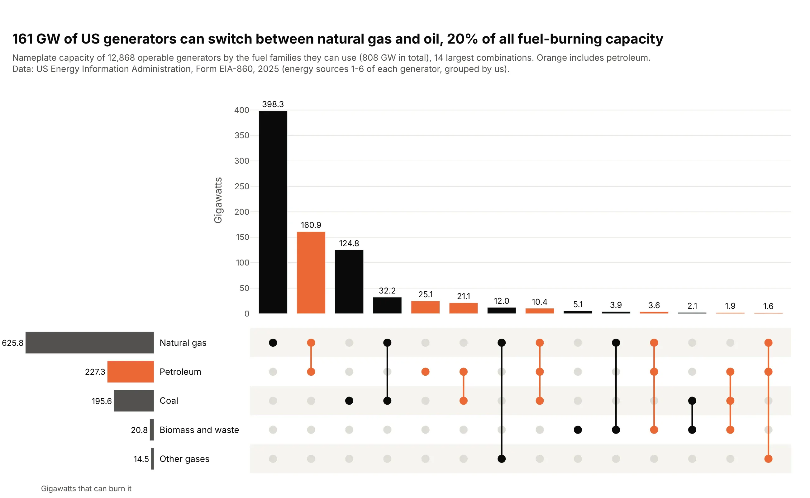
UpSet plot of the fuels 12,868 US generators can burn, with bars in gigawatts. Natural gas only is 398.3 GW, natural gas plus petroleum (orange) is 160.9 GW and coal only is 124.8 GW; set bars show 625.8 GW can burn gas and 227.3 GW petroleum

Capabilities, weighted by size. Summing nameplate capacity instead of counting units shows that 161 GW of US generators can switch between natural gas and oil, 20% of all fuel-burning capacity. Data: US EIA, Form EIA-860, 2025.

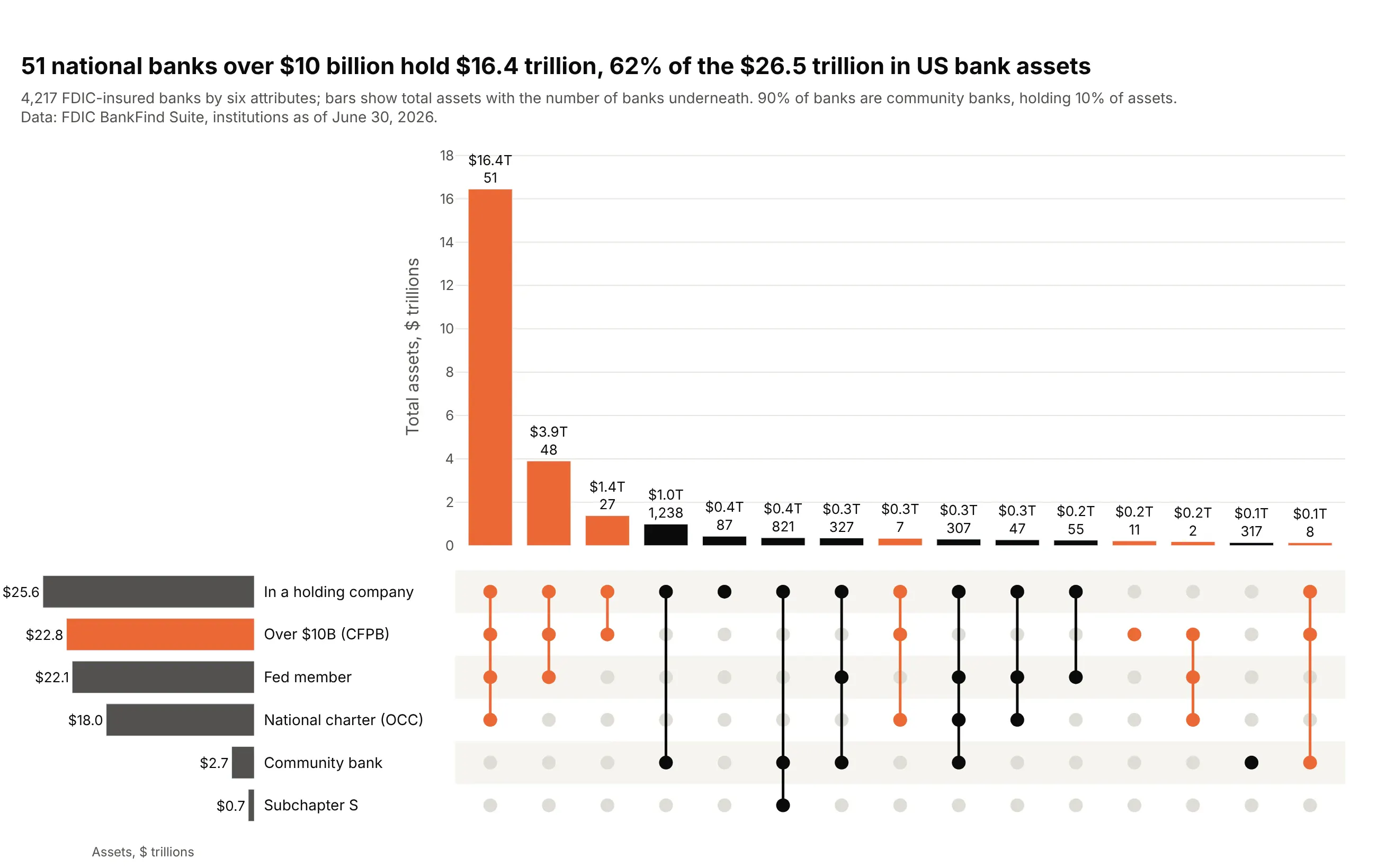
UpSet plot of 4,217 FDIC-insured banks by six attributes, with bars in trillions of dollars of assets and the number of banks under each value. The first bar, 51 national banks over $10 billion in holding companies that are Fed members, holds $16.4 trillion; 1,238 community banks in holding companies hold $1.0 trillion

Two numbers per combination. The bars are assets and the text adds the bank count, so it shows that 51 big national banks hold $16.4 trillion, 62% of US bank assets, while 90% of banks are community banks. Data: FDIC BankFind Suite, June 30, 2026.

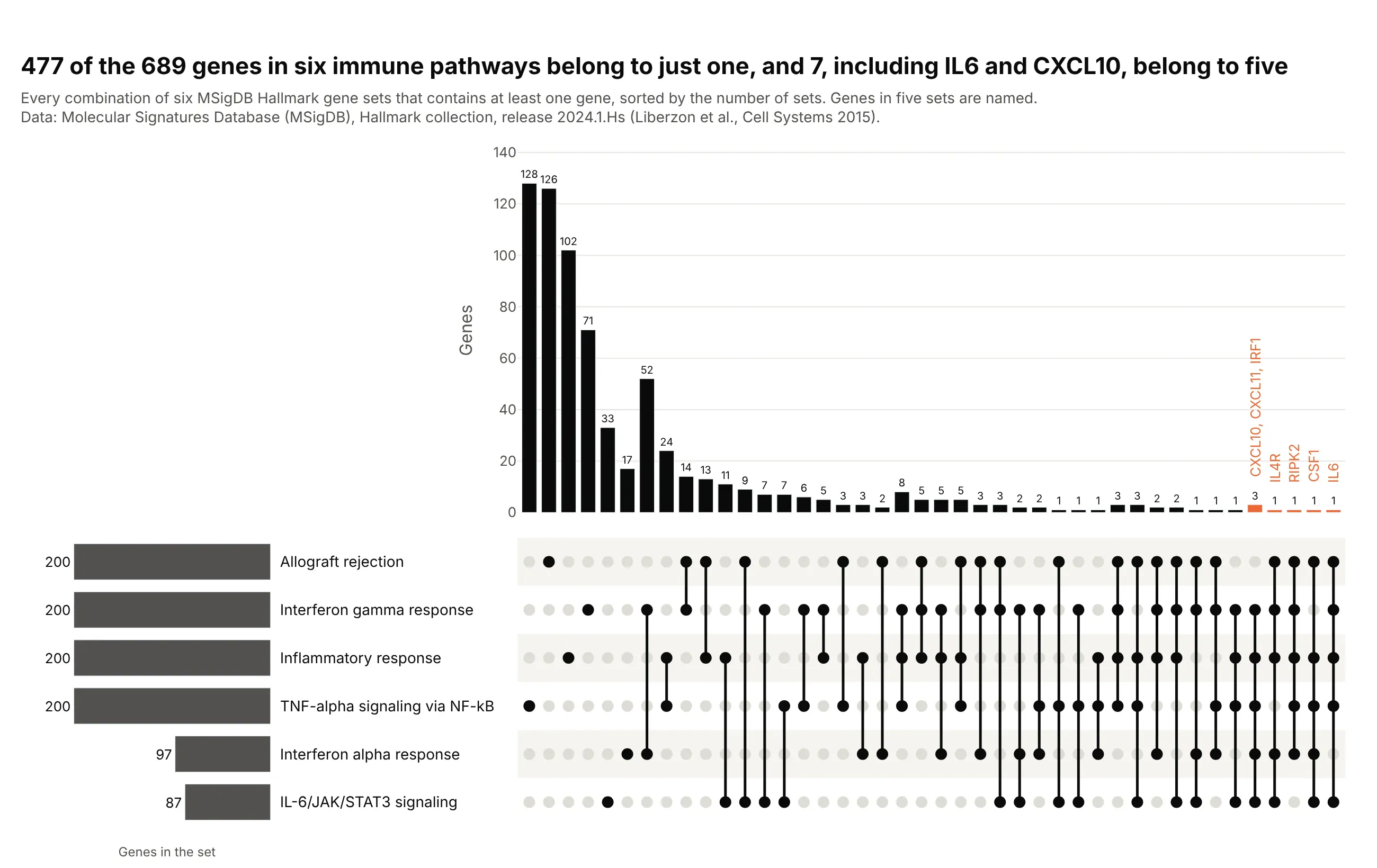
UpSet plot of 689 genes in six MSigDB Hallmark immune gene sets, sorted by degree. The first six bars are genes in one set only (128, 126, 102, 71, 33 and 17), and the last five orange bars are genes in five sets, labeled CXCL10, CXCL11, IRF1, IL4R, RIPK2, CSF1 and IL6

Gene sets. Sorted by degree, it shows that 477 of 689 genes belong to just one of six immune pathways and seven, including IL6 and CXCL10, belong to five. Data: MSigDB Hallmark gene sets, release 2024.1.Hs.

A short history

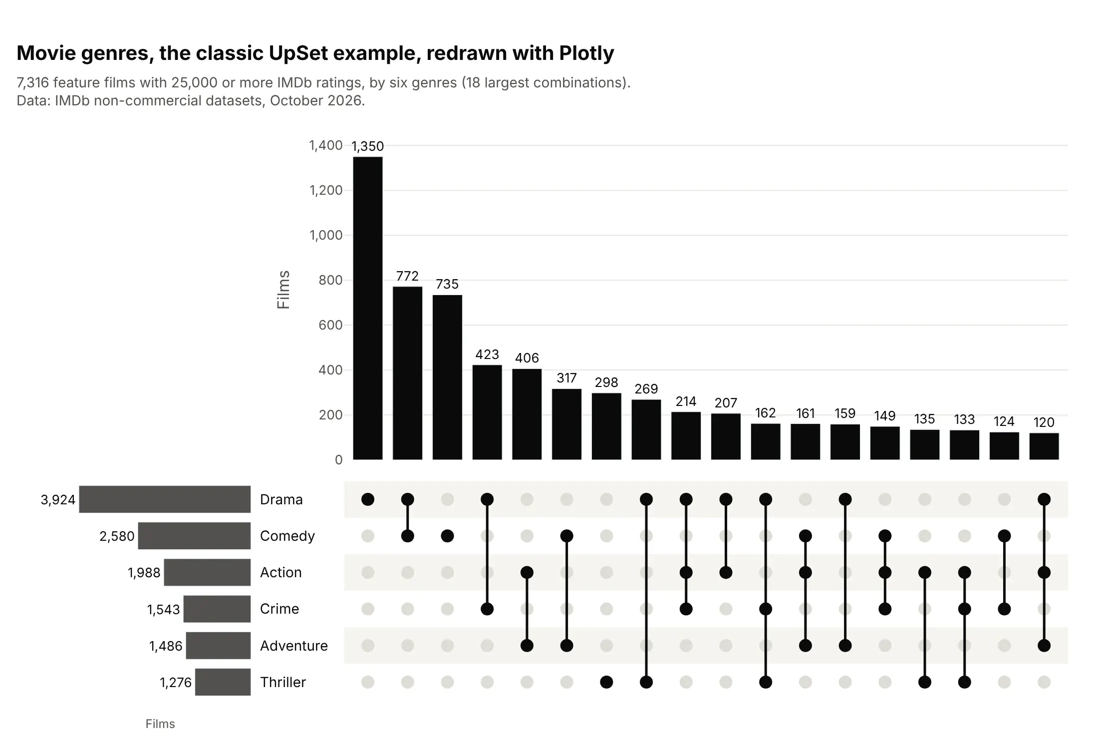
John Venn published his diagrams in 1880 (Venn 1880, doi:10.1080/14786448008626877), and they work for two or three sets. Alexander Lex, Nils Gehlenborg and colleagues introduced the UpSet plot in 2014 as a scalable alternative (Lex et al. 2014, doi:10.1109/TVCG.2014.2346248), and the R package UpSetR made it common in genomics (Conway, Lex and Gehlenborg 2017, doi:10.1093/bioinformatics/btx364). UpSetR's standard example is movie genres from GroupLens's MovieLens data. Here is the same idea redrawn with Plotly on IMDb's genre data:

UpSet plot redrawn with Plotly of 7,316 feature films with 25,000 or more IMDb ratings by six genres. Drama only is the largest combination at 1,350 films, then drama plus comedy (772) and comedy only (735)

Alternatives to an UpSet plot

Here's the same data on four conditions drawn five ways. Some are better for the question, some worse, some just different:

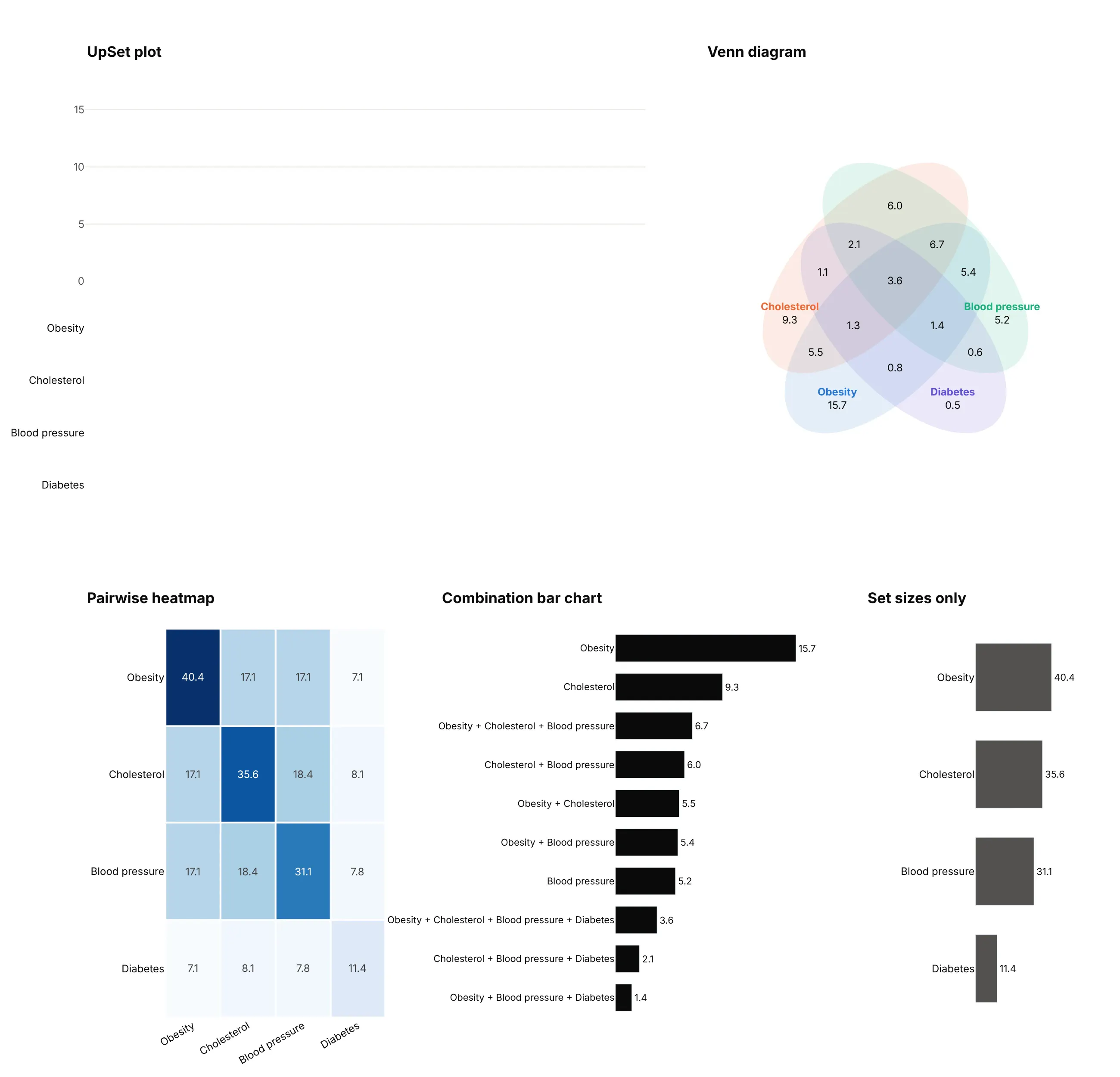
The same four conditions (obesity, high cholesterol, high blood pressure, diabetes) as an UpSet plot, a four-ellipse Venn diagram with 15 region values such as 15.7% for obesity only and 3.6% for all four, a pairwise heatmap with 17.1% of adults having both obesity and high cholesterol, a sorted bar chart of named combinations, and a bar chart of the four set sizes alone

Venn diagram (works for two or three sets, worse past that). Four sets need ellipses and 15 regions, so you can't compare region sizes and it's hard to find a given combination. Five or more sets don't fit.
Pairwise heatmap (different). Shows the overlap of every pair, here 17.1% of adults with both obesity and high cholesterol, and scales to dozens of sets. It can't show combinations of three or more.
Combination bar chart (works too). A sorted bar chart with the combination written out as the label is an UpSet plot without the matrix. It's fine for a few sets, but the labels get long and you can't scan by set.
Set sizes only (worse). A bar chart of each set's total hides the overlap, which is the question.

How to make an UpSet plot

With AI

ChatGPT, Claude Code, GitHub Copilot, Cursor and other AI tools are excellent at writing Plotly code. Name Plotly in the prompt, describe the three parts and how to draw them, and list the checks you want:

Make a plotly UpSet plot from conditions.csv (one row per person, 0/1 columns: obesity,
high_bp, high_chol, diabetes, arthritis, heart_disease; a survey weight column).

- Use make_subplots with a bar chart of intersection sizes on top,
  a dot matrix under it (go.Scatter markers, gray when a set is absent, dark when present,
  joined by a vertical line), and horizontal bars of set sizes on the left growing leftward.
- Count exclusive intersections (each row lands in exactly one combination), weighted by the
  survey weight, as a % of all rows. Leave out the empty combination.
- Sort by size and show the 20 largest. Largest set on the top row of the matrix.
- Color every combination that includes diabetes orange, in the bars and the matrix.
- Put the value on each bar, Inter font, white background, a title that states the takeaway.
- Check that the intersection sizes add up to 100% minus the empty combination.

With Plotly Studio

Plotly Studio is a desktop app where you point an AI at a dataset and it builds charts and a Dash app around your questions. Ask for an UpSet plot the same way:

Make an UpSet plot of the six condition columns: bars for the 20 most common exact combinations, a dot matrix under them showing which conditions each bar is, and set sizes on the left. Add a dropdown to highlight one condition.

Make an UpSet plot in Python or JavaScript

This is the code AI tools write under the hood. In Python, this short version of the helper counts the combinations with groupby and draws the three parts:

import pandas as pd
import plotly.graph_objects as go
from plotly.subplots import make_subplots


def make_upset(df, sets, max_bars=20):
    """df: one row per item, one True/False column per set."""
    inter = (df.groupby(sets).size().reset_index(name="size")
               .query(" or ".join(f"`{s}`" for s in sets))          # drop the empty set
               .sort_values("size", ascending=False).head(max_bars).reset_index(drop=True))
    order = sorted(sets, key=lambda s: df[s].sum())                    # largest set on top
    fig = make_subplots(rows=2, cols=2, column_widths=[0.2, 0.8], row_heights=[0.6, 0.4],
                        specs=[[None, {}], [{}, {}]], shared_xaxes=True,
                        vertical_spacing=0.03, horizontal_spacing=0.12)
    fig.add_bar(x=inter.index, y=inter["size"], text=inter["size"], textposition="outside",
                marker_color="#0b0b0b", row=1, col=2)
    for i, r in inter.iterrows():
        ys = [order.index(s) for s in sets if r[s]]
        fig.add_scatter(x=[i] * len(order), y=list(range(len(order))), mode="markers",
                        marker=dict(size=12, color="#dddcd6"), row=2, col=2)
        fig.add_scatter(x=[i] * len(ys), y=ys, mode="lines+markers", line_color="#0b0b0b",
                        marker=dict(size=12, color="#0b0b0b"), row=2, col=2)
    fig.add_bar(y=order, x=[df[s].sum() for s in order], orientation="h",
                marker_color="#52514e", row=2, col=1)
    fig.update_xaxes(visible=False, col=2)
    fig.update_xaxes(autorange="reversed", row=2, col=1)
    fig.update_yaxes(visible=False, row=2, col=2)
    fig.update_yaxes(side="right", row=2, col=1)
    fig.update_layout(showlegend=False, template="simple_white")
    return fig


df = pd.read_csv("conditions.csv")   # columns: Obesity, High cholesterol, High blood pressure, ...
fig = make_upset(df.astype(bool), ["Obesity", "High cholesterol", "High blood pressure", "Diabetes"])
fig.show()

The full make_upset() used for every chart in this guide adds weight= (sum a column instead of counting rows), sort_by="degree", highlight= (color one set), values= (a box plot per bar) and set_order=.

In JavaScript, plotly.js takes the same three pieces as plain traces. This one draws three conditions from NHANES as a share of US adults:

<div id="chart"></div>
<script src="https://cdn.plot.ly/plotly-4.1.1.min.js"></script>
<script>
  const sets = ["Obesity", "High cholesterol", "High blood pressure"];  // rows, bottom to top
  const combos = [[1,0,0], [0,1,0], [1,1,1], [0,1,1], [1,0,1], [1,1,0], [0,0,1]];
  const sizes = [16.5, 10.4, 10.3, 8.1, 6.8, 6.8, 5.8];  // % of US adults, NHANES 2021-2023
  const x = combos.map((_, i) => i);
  const dots = combos.flatMap((c, i) => c.map((on, j) => ({x: i, y: j, on})));
  const lines = combos.flatMap((c, i) => {
    const ys = c.flatMap((on, j) => on ? [j] : []);
    return [{x: i, y: Math.min(...ys)}, {x: i, y: Math.max(...ys)}, {x: null, y: null}];
  });
  Plotly.newPlot("chart", [
    {type: "bar", x, y: sizes, text: sizes, textposition: "outside", cliponaxis: false, marker: {color: "#0b0b0b"}},
    {x: dots.map(d => d.x), y: dots.map(d => d.y), yaxis: "y2", mode: "markers",
     marker: {size: 14, color: dots.map(d => d.on ? "#0b0b0b" : "#dddcd6")}},
    {x: lines.map(d => d.x), y: lines.map(d => d.y), yaxis: "y2", mode: "lines",
     line: {color: "#0b0b0b", width: 3}}
  ], {
    showlegend: false, margin: {l: 150},
    xaxis: {visible: false},
    yaxis: {domain: [0.45, 1], title: {text: "% of US adults"}},
    yaxis2: {domain: [0, 0.4], tickvals: [0, 1, 2], ticktext: sets, range: [-0.5, 2.5], zeroline: false, showgrid: false}
  });
</script>

Count exclusive intersections, where each item lands in exactly one combination, so the bars add up to the number of items that are in at least one set.

Share it

Every Plotly chart has a Share chart button (the cloud icon in its toolbar) that uploads it to Plotly Cloud and gives you a link. Only you can see it until you change its visibility.

For a live app, put the chart in a Dash app and publish it with the Plotly Cloud CLI. Coding agents can run these commands for you:

pip install "dash[cloud]"
plotly user login
plotly app publish

If your data has to stay in your own cloud or data center, publish to Dash Enterprise instead.

Dos and don'ts

Most of the work is choosing which combinations to show and in what order. Here is the same NHANES data both ways.

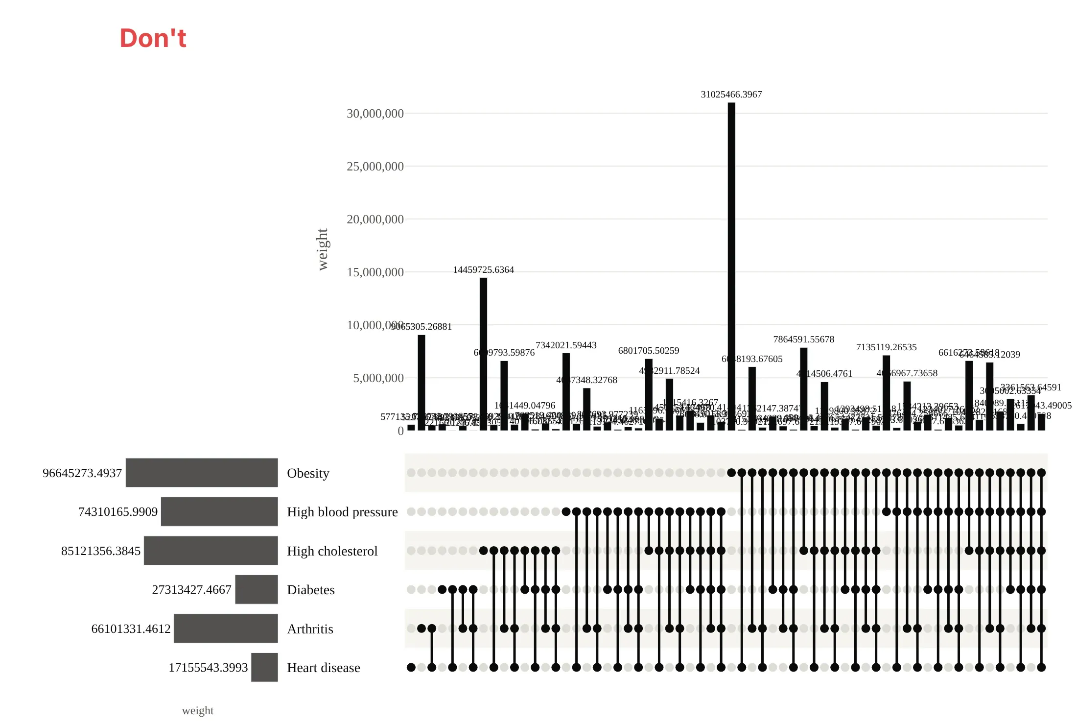
Don't draw every combination in the order groupby returns them, print raw unformatted numbers that overlap, or leave the default serif font:

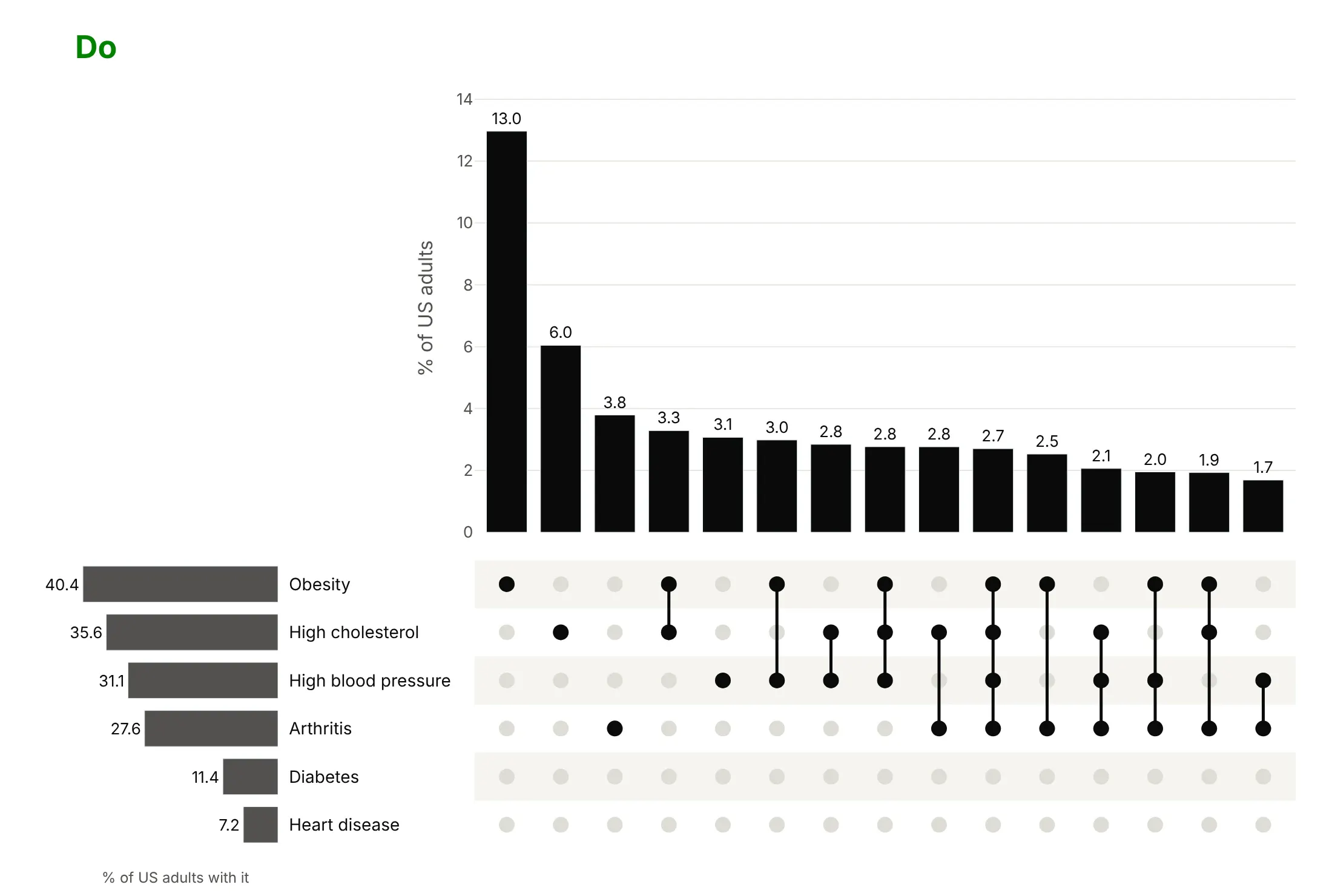
An UpSet plot of the six conditions with all 63 combinations in binary order, so the largest bar sits in the middle, raw survey weights such as 31025466.3967 printed on top of each other above the bars, and a serif font

Do sort by size, keep the 15 largest, and show values as a formatted share:

The same data as a sorted UpSet plot of the 15 largest combinations, labeled with the share of US adults such as 13.0 for obesity alone, in the Inter font

Sorting, highlighting and distributions

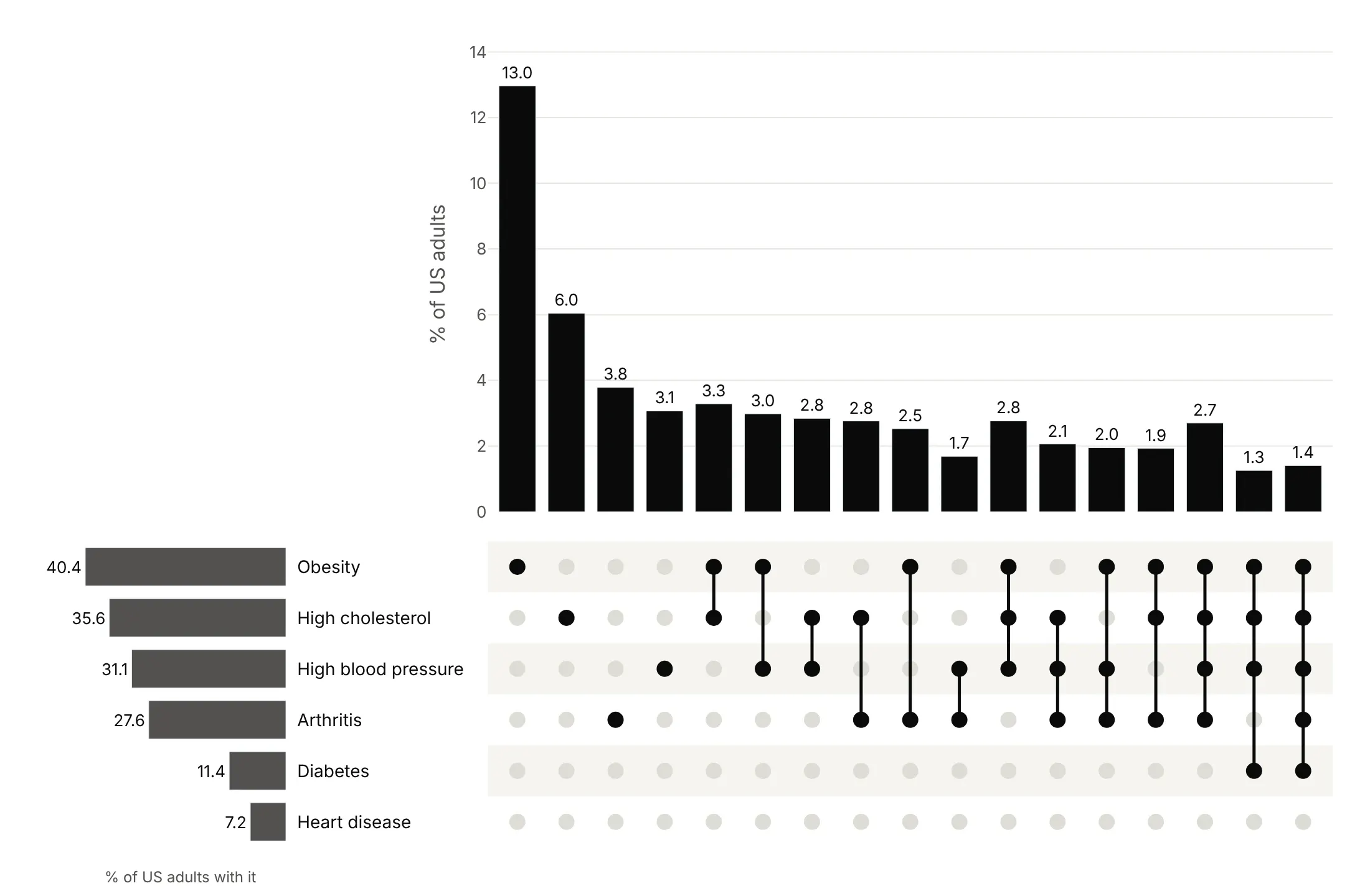
Sort by size to find the most common combinations first. This is the right default.

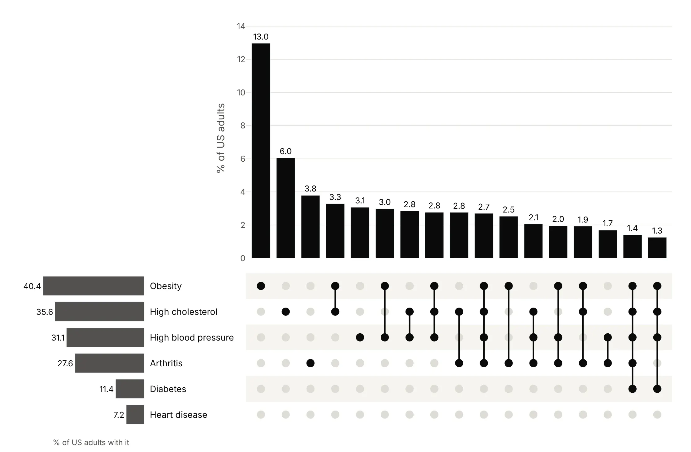
UpSet plot of the conditions with the 17 combinations of at least 1% of adults, sorted from 13.0% (obesity alone) down

Sort by degree to read single conditions first, then pairs, then triples. Use it when the number of sets is the point.

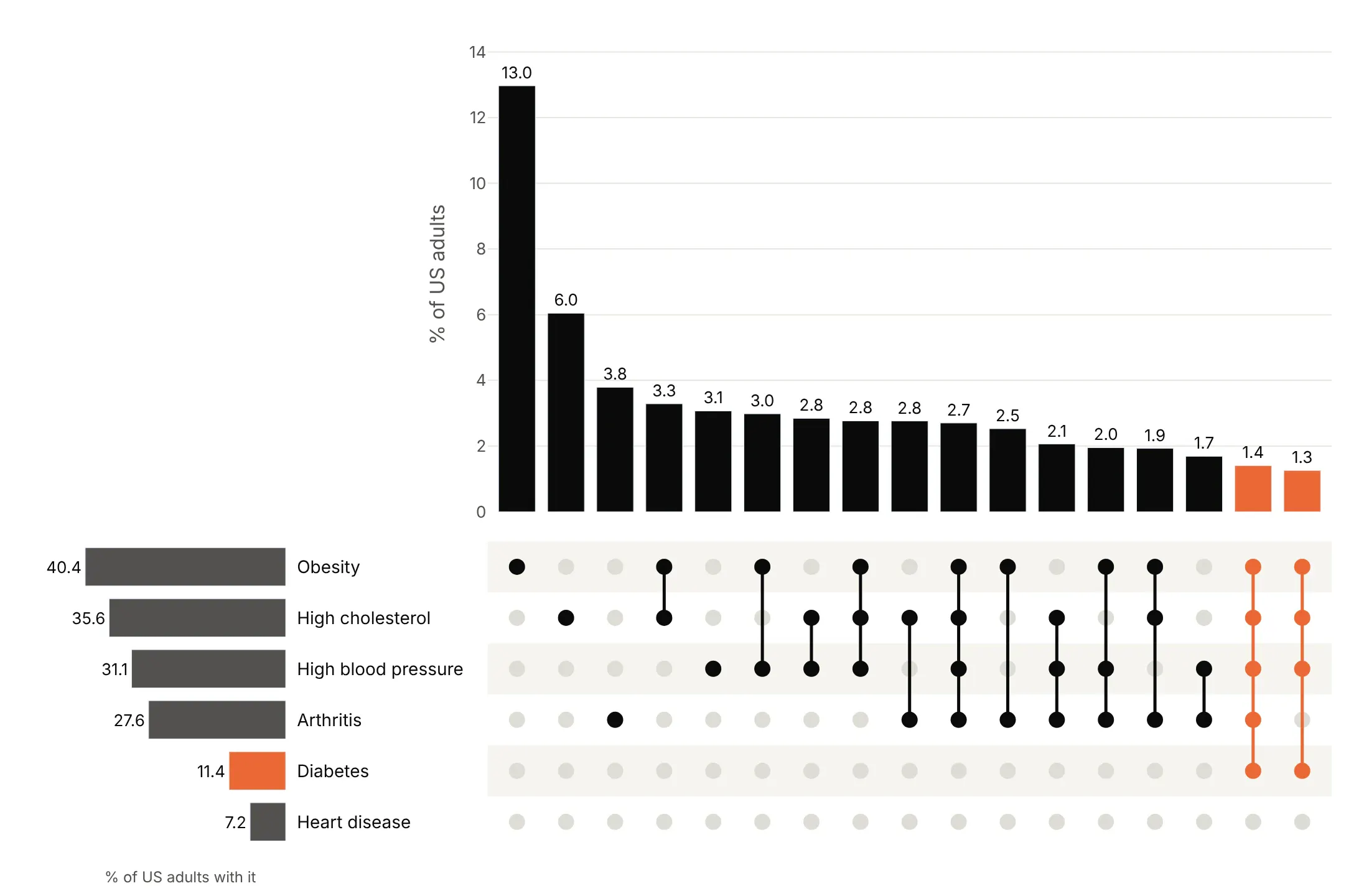
The same 17 combinations sorted by degree: the four single conditions first, then six pairs, four triples, two combinations of four and one of five conditions

Highlight one set to follow it through every combination. Here every combination with diabetes is orange.

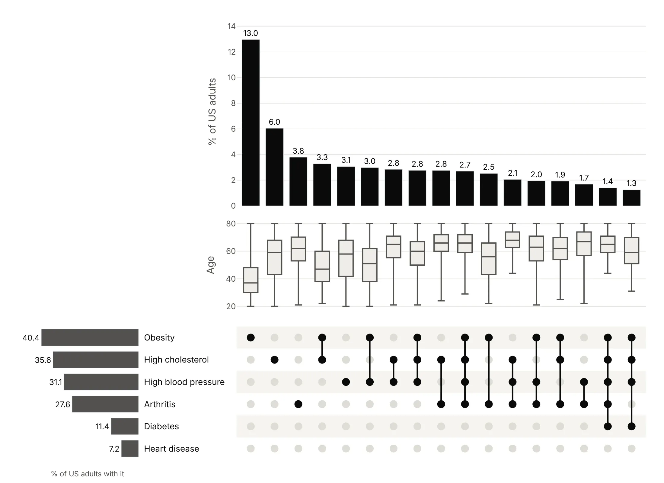
The same UpSet plot with the two combinations of at least 1% that include diabetes in orange in the bars and the matrix, and the diabetes set bar in orange

Add a distribution per intersection to compare a variable across combinations. Here a box plot of age shows that people with more conditions are older.

The same UpSet plot with a row of box plots of age between the bars and the matrix; the median age is 37 for obesity alone and 60 to 68 for the combinations of three conditions

Checklist

Write a title that states the takeaway, with the number.
Sort by size (or by degree when that's the story) and show the 15-25 largest combinations.
Say in the subtitle how many combinations or items are left out, including the empty one.
Put the value on each bar, formatted, and use the same unit on the set bars.
Use one color for the bars and a second only to highlight one set.

Don't

Use a Venn diagram for four or more sets.
Show combinations in arbitrary order.
Mix up inclusive counts (everyone with diabetes) and exclusive ones (diabetes and nothing else) on the bars.
Rely on hover to say which sets a bar is; the matrix must say it.

Options to customize

These are the Plotly pieces that matter for building an UpSet plot. The references are the subplots, bar chart and scatter documentation.

make_subplots(rows, cols, specs, shared_xaxes): lays out the bars, the matrix and the set bars so the columns line up; specs=[[None, {}], [{}, {}]] leaves the top-left empty.
column_widths, row_heights: how much room the set bars and the matrix get.
horizontal_spacing: room for the set names between the set bars and the matrix.
go.Bar(x, y, text, texttemplate): the intersection sizes, with the value on each bar.
textposition="outside", cliponaxis=False: values above the bars without clipping.
go.Scatter(mode="markers"): the matrix dots; one trace of gray dots for every cell and one of dark dots for members.
go.Scatter(mode="lines") with None gaps: the vertical lines joining the dots of each combination, all in one trace.
marker.color as a list: one color per bar or dot, for highlighting a set.
go.Bar(orientation="h") with xaxis.autorange="reversed": set sizes growing to the left, toward the set names.
yaxis.side="right", ticklabelstandoff: puts the set names between the set bars and the matrix.
add_hrect: light stripes behind every other matrix row.
yaxis.type="log": a log scale when one combination dwarfs the rest.
go.Box(x, y): a distribution per intersection in an extra subplot row.
customdata, hovertemplate: the names of the sets in each combination on hover.

More UpSet plot examples

Six more UpSet plots built from real public data, each with its source, the technique that makes it work and a prompt to rebuild it.

1. Side effects reported for semaglutide

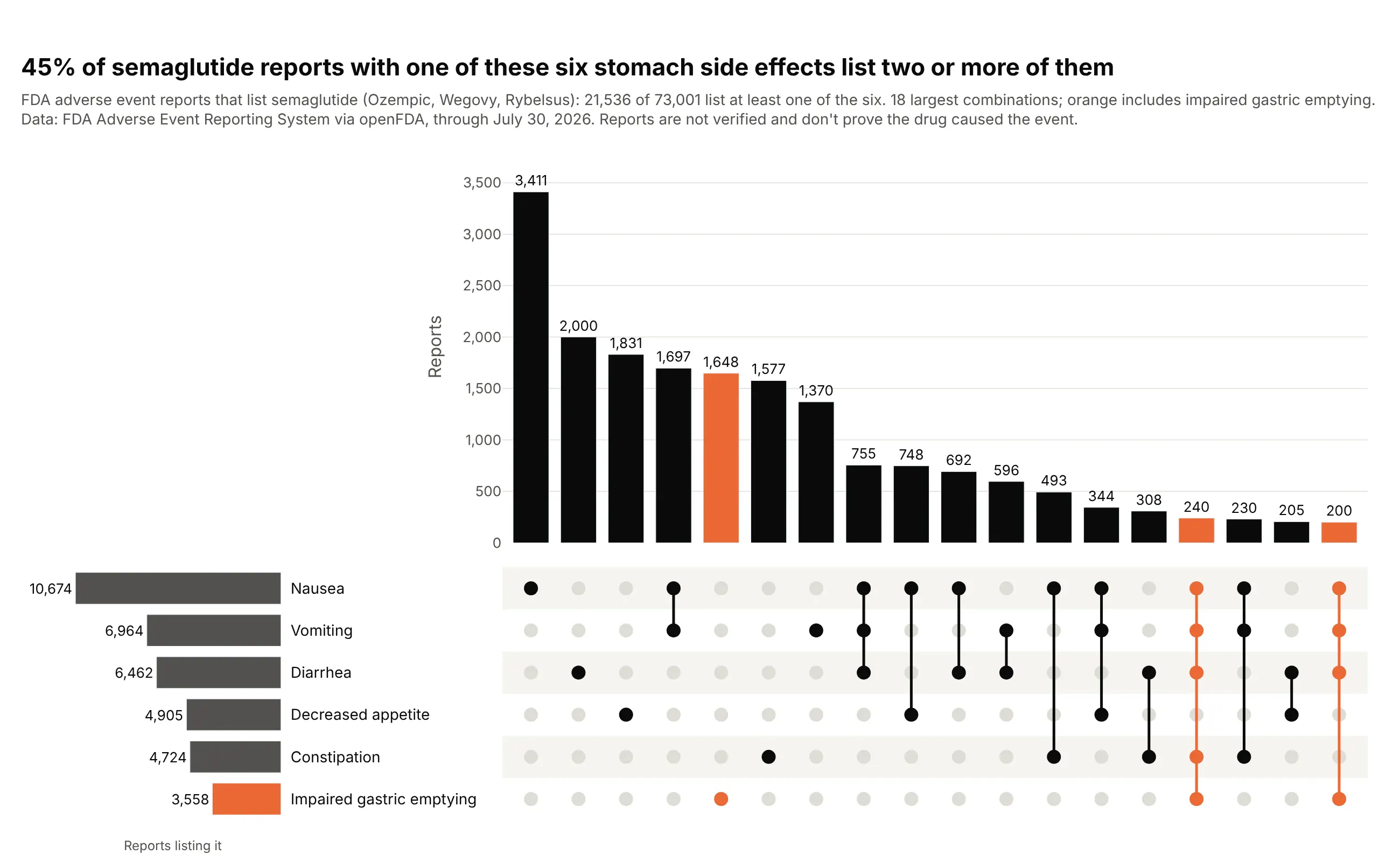
UpSet plot of FDA adverse event reports listing semaglutide by six stomach-related reactions. Nausea alone is the largest combination (3,411 reports), then diarrhea alone (2,000), decreased appetite alone (1,831) and nausea plus vomiting (1,697); impaired gastric emptying alone (1,648) is orange

Of 73,001 FDA adverse event reports that list semaglutide, 21,536 mention at least one of these six stomach side effects, and 45% of those list two or more. Nausea alone is the most common (3,411 reports). Reports are unverified and don't prove causation. Data: FDA FAERS via openFDA, through July 30, 2026.

Tip: the API returns counts per combination rather than one row per report, so weight="reports" sums a count column instead of counting rows.

Get the data from the FDA Adverse Event Reporting System through the openFDA drug event API
(api.fda.gov/drug/event.json), reports whose drug list includes semaglutide, and shape it into
a table with one row per exact combination of six reactions (columns: Nausea, Vomiting, Diarrhea,
Constipation, Decreased appetite, Impaired gastric emptying as 0/1, reports). Count reports with
all reactions in each subset, then use inclusion-exclusion to get exclusive counts.

Make a plotly UpSet plot (make_subplots with go.Bar and go.Scatter): bars = reports per exact
combination, 18 largest, sorted by size; combinations with impaired gastric emptying in orange.
Note in the subtitle that reports are unverified.

2. Where Phase 3 trials run

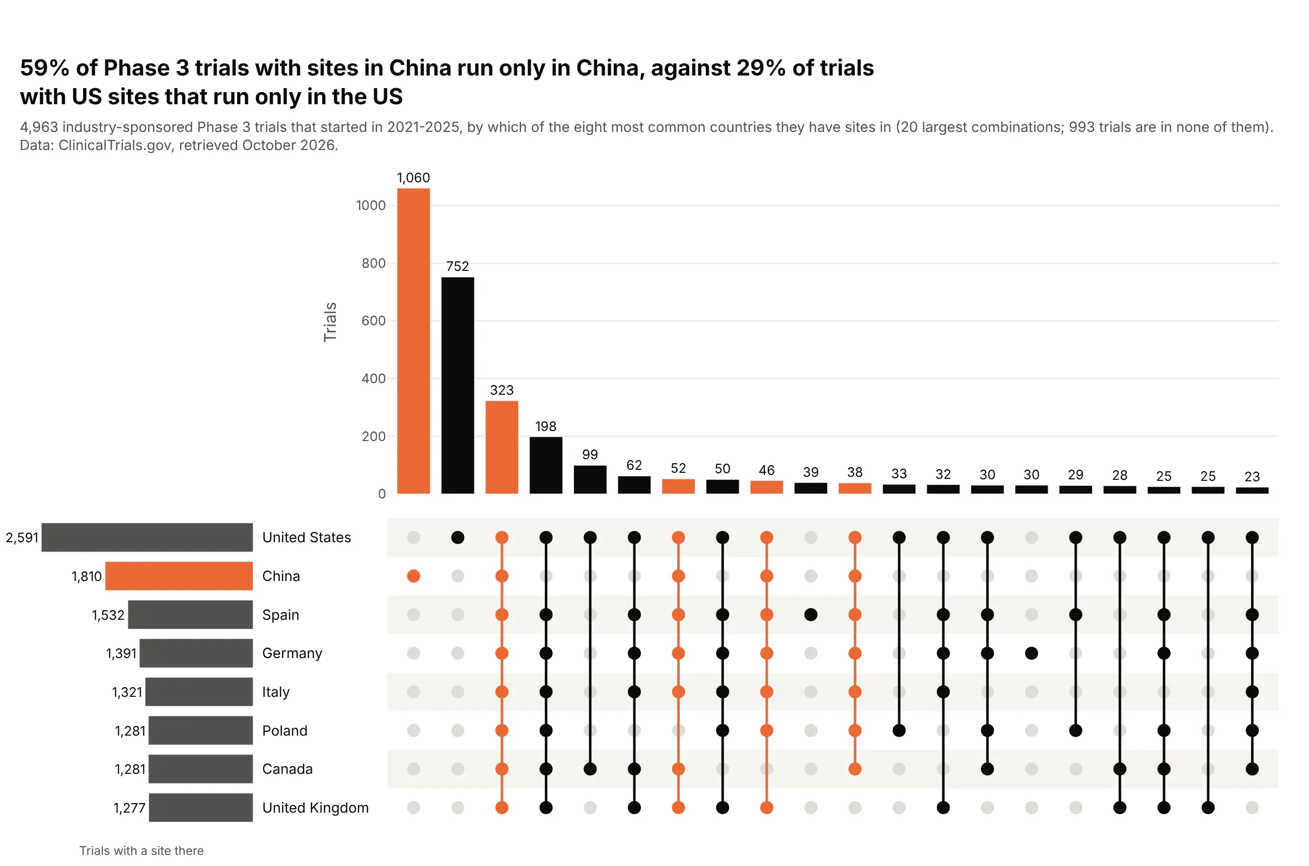
UpSet plot of 4,963 industry Phase 3 trials started 2021-2025 by eight countries. China only is the largest bar (1,060 trials, orange), US only is 752, and trials in all eight countries are 323

Of 4,963 industry Phase 3 trials started in 2021-2025, 1,060 run only in China, the largest single combination. That's 59% of trials with sites in China, against 29% of trials with US sites that run only in the US, and 323 trials run in all eight countries. Data: ClinicalTrials.gov API v2.

Tip: with eight sets there are 255 possible combinations, so max_bars=20 keeps the largest and the subtitle says how many trials are in none of the eight.

Get the data from the ClinicalTrials.gov API v2 (clinicaltrials.gov/api/v2/studies), industry-sponsored
Phase 3 trials that started 2021-2025, and shape it into a table (columns: nct_id, enrollment,
n_countries, and 0/1 columns for the eight countries with the most trials).

Make a plotly UpSet plot of the 20 largest country combinations, sorted by size, with every
combination that includes China in orange and the set sizes on the left.

3. Power plants that mix technologies

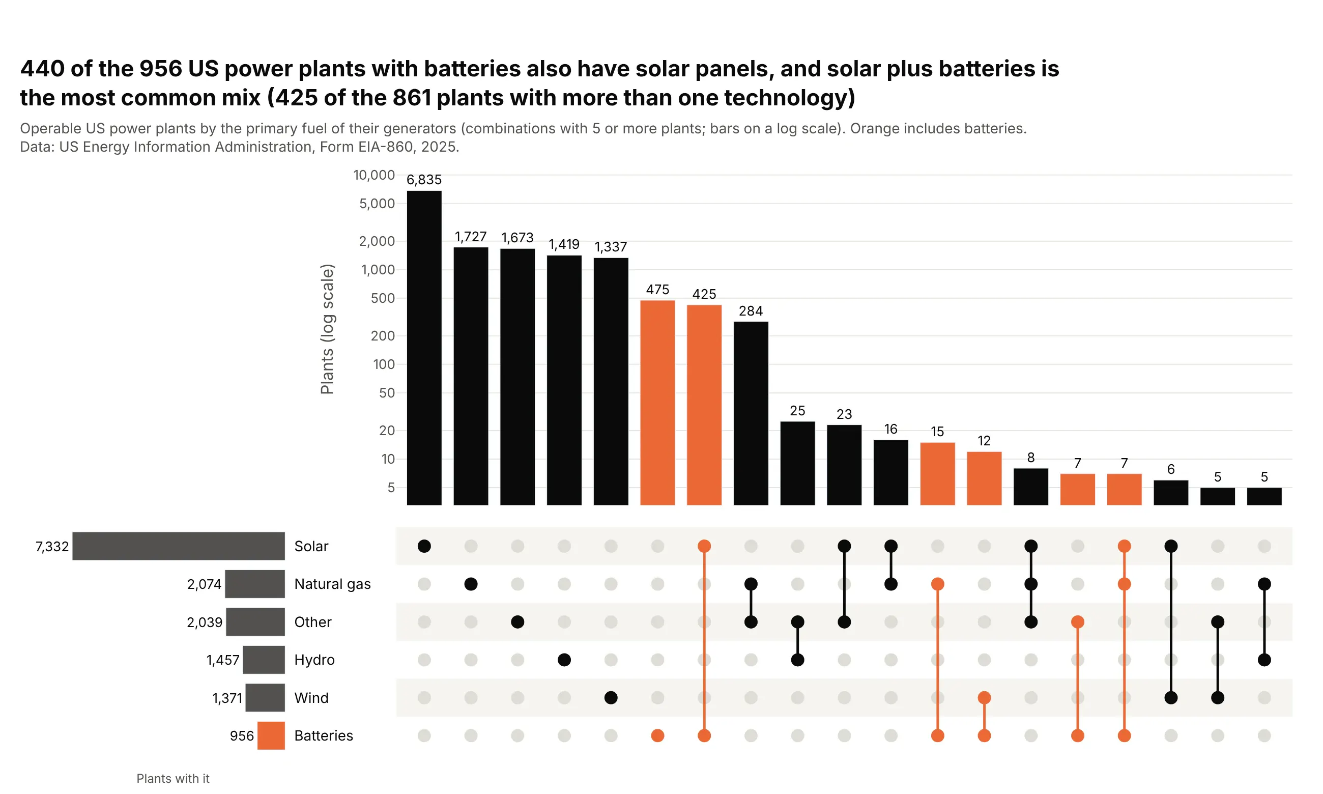
UpSet plot of 14,327 US power plants by technology on a log scale. Solar only is 6,835 plants; batteries only (475) and solar plus batteries (425) are orange; natural gas plus other is 284

Almost every US power plant has one technology, so the interesting part is the small columns. 440 of the 956 plants with batteries also have solar panels, and solar plus batteries is the most common mix (425 of the 861 plants with more than one technology). Data: US EIA, Form EIA-860, 2025.

Tip: yaxis.type="log" on the bar row keeps the 6,835 solar-only plants from flattening the hybrids.

Get the data from the US EIA's Form EIA-860 2025 generator file (eia.gov/electricity/data/eia860,
3_1_Generator_Y2025.xlsx, sheet Operable) and shape it into a table with one row per plant
(columns: plant_code, state, capacity_mw, and 0/1 columns Solar, Batteries, Wind, Natural gas,
Hydro, Other from each generator's Energy Source 1).

Make a plotly UpSet plot of plants by technology mix: combinations with 5+ plants, sorted by size,
bars on a log scale, combinations that include batteries in orange.

4. Major disasters by county

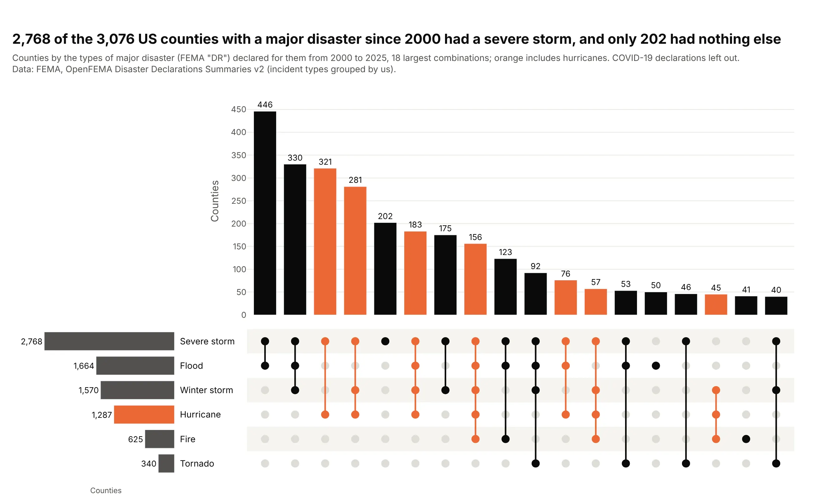
UpSet plot of 3,076 US counties by the types of major disaster declared since 2000. Severe storm plus flood is the largest combination (446 counties), and combinations with hurricanes are orange

2,768 of the 3,076 counties with a major disaster declaration since 2000 had a severe storm, and only 202 had nothing else. Severe storm plus flood is the most common pair at 446 counties. Data: FEMA, OpenFEMA Disaster Declarations Summaries v2.

Tip: the set bars on the left show at a glance that severe storm is much larger than the other five sets, which the intersection bars alone hide.

Get the data from FEMA's OpenFEMA Disaster Declarations Summaries v2 API (fema.gov/api/open),
major disaster declarations ("DR") from 2000 to 2025 in the 50 states and DC, and shape it into a
table with one row per county (columns: fips, state, county, declarations, and 0/1 columns
Severe storm, Flood, Winter storm, Hurricane, Fire, Tornado; leave out COVID-19).

Make a plotly UpSet plot of the 18 largest combinations, sorted by size, with every combination
that includes hurricanes in orange.

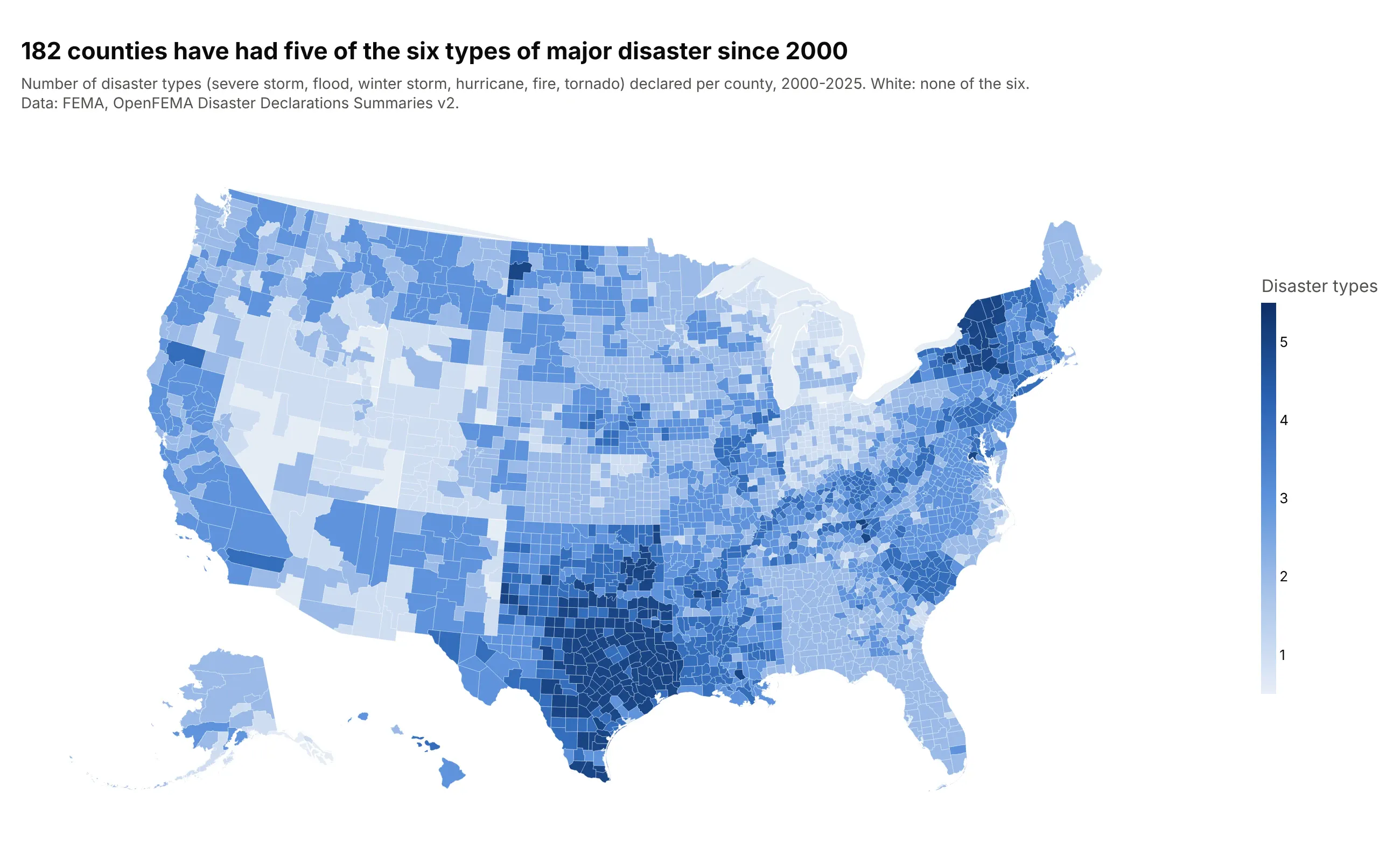
Another way to see it: a county map shows where the hazards pile up, with 182 counties hit by five of the six types (135 of them in Texas), but it can't show which combination each county had.

Map of US counties shaded by how many of six disaster types have been declared there since 2000, darkest across Texas, Oklahoma and New York, where counties had five types

5. How exoplanets are detected

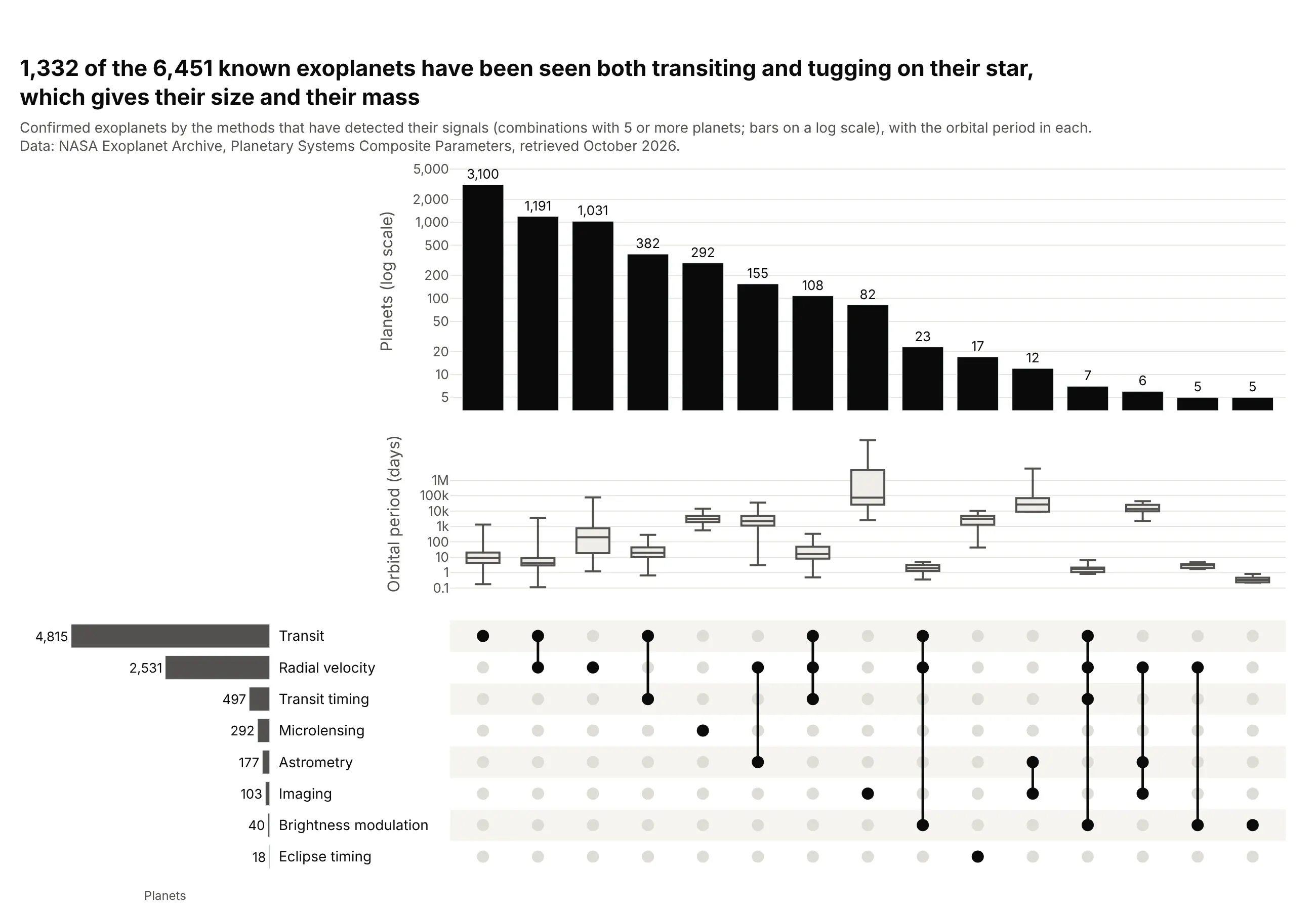
UpSet plot of 6,451 confirmed exoplanets by detection method on a log scale, with a box plot of orbital period per combination. Transit only is 3,100 planets with a median period of about 9 days, transit plus radial velocity is 1,191, and imaging-only planets have periods in the tens of thousands of days

1,332 of the 6,451 known exoplanets have been seen both transiting their star and tugging on it, which gives both their size and their mass. The box plots show why methods differ: transit-only planets have a median orbit of 9.0 days, while radial velocity alone finds planets with a median orbit of 200 days. Data: NASA Exoplanet Archive.

Tip: values="pl_orbper" with a log axis on the box row shows a distribution that spans six orders of magnitude under each bar.

Get the data from the NASA Exoplanet Archive's Planetary Systems Composite Parameters table
(exoplanetarchive.ipac.caltech.edu, TAP query on pscomppars) and shape it into a table
(columns: pl_name, disc_year, discoverymethod, pl_orbper, and 0/1 columns from tran_flag, rv_flag,
ima_flag, micro_flag, ttv_flag, ast_flag, etv_flag, ptv_flag, obm_flag).

Make a plotly UpSet plot of detection-method combinations with 5+ planets: bars on a log scale,
then a row of box plots of orbital period per combination (log axis), then the dot matrix.

6. Python versions declared by popular packages

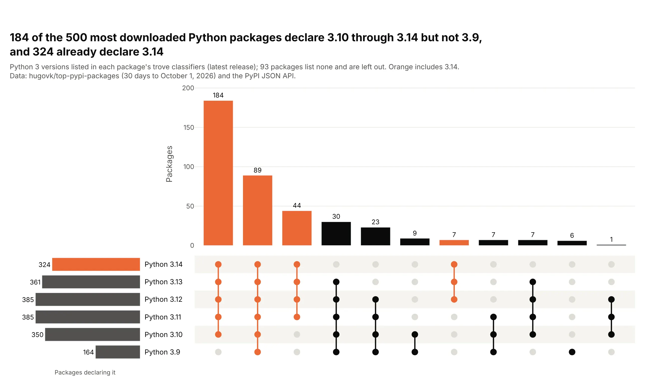
UpSet plot of the Python 3 versions declared by the 500 most downloaded PyPI packages, with set rows in version order from 3.14 on top to 3.9. Python 3.10 through 3.14 is the largest combination (184 packages), all six versions is 89, and combinations that include 3.14 are orange

Of the 500 most downloaded PyPI packages, 184 declare Python 3.10 through 3.14 but not 3.9, and 324 already declare 3.14. Most combinations are runs of consecutive versions, which show as unbroken vertical lines in the matrix; 93 packages declare no versions in their classifiers. Data: hugovk/top-pypi-packages and the PyPI JSON API.

Tip: sets with a natural order keep it with set_order=, so runs of versions read as solid lines instead of being shuffled by set size.

Get the data from hugovk's top PyPI packages list (hugovk.github.io/top-pypi-packages) and the
PyPI JSON API (pypi.org/pypi/<name>/json) for the top 500 packages, and shape it into a table
(columns: rank, project, requires_python, and 0/1 columns py3.9 ... py3.14 from the
"Programming Language :: Python :: 3.X" classifiers).

Make a plotly UpSet plot of version combinations with the set rows in version order (3.14 on top),
sorted by size, combinations that include 3.14 in orange.

UpSet Plots - A Complete Guide (with 10 Examples)

What is an UpSet plot?

A short history

Alternatives to an UpSet plot

How to make an UpSet plot

With AI

With Plotly Studio

Make an UpSet plot in Python or JavaScript

Share it

Dos and don'ts

Sorting, highlighting and distributions

Checklist

Options to customize

More UpSet plot examples

1. Side effects reported for semaglutide

2. Where Phase 3 trials run

3. Power plants that mix technologies

4. Major disasters by county

5. How exoplanets are detected

6. Python versions declared by popular packages

FAQ

What is an UpSet plot?

How do you read an UpSet plot?

Why use an UpSet plot instead of a Venn diagram?

How do I make an UpSet plot in Python with Plotly?

What is the difference between inclusive and exclusive intersections?

How many sets and combinations can an UpSet plot show?

Can I add a distribution or a second variable to an UpSet plot?

Can I make an UpSet plot in Excel?