Plotly team

July 28, 2026

Serving a month of Polymarket data: scaling, metering, and MCP on Plotly Cloud

Polymarket publishes its full orderbook as a public dataset: every price update on every active prediction market, stamped to the millisecond. One month is ~16 billion events and 500 GB of compressed Parquet. The companion Polars blog post covers how that raw feed is decoded and aggregated at scale on Polars Cloud — the same query running unchanged on one hour locally and a month in the cloud.

This month, the Polars Cloud team and Plotly team have partnered to take this dataset to production using a modern data stack: Big data analytics backed by Polars Cloud, a data app built using Dash, and app hosting and scaling powered by Plotly Cloud.

In this post, we’ll cover what the process of hosting and distributing our Polymarket Dash app looked like, and the features we added to the app by publishing it to Plotly Cloud – specifically, enabling AI agents to interface with the underlying dataset without any additional development. A shaped dataset still needs an app that handles large data, stays responsive under traffic, and increasingly answers to AI agents as well as people — a lot of infrastructure to stand up yourself. On Plotly Cloud, you don't. We built the dashboard as an ordinary Dash app and published it; three platform capabilities did the ops work:

Large-data serving — a high-performance store the app reads at runtime, on a machine Cloud sizes to hold the working set.
Compute modes and custom machine sizes — one control surface to keep the app awake and scale its machine, billed hourly from a shared credit pool.
MCP auth, handled by the platform — turn the app into an MCP server for agents, secured by its existing access controls. No auth code.

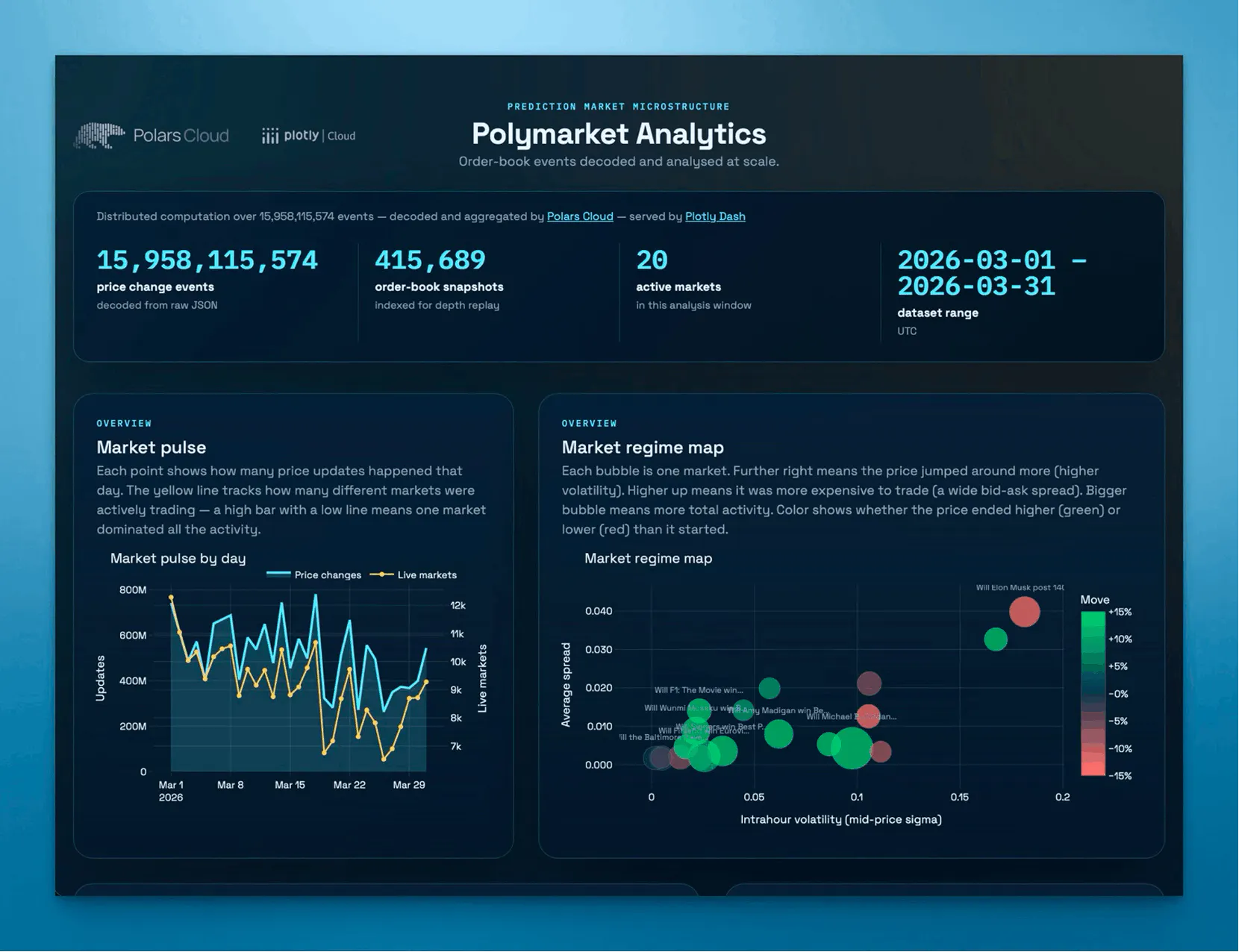
The end result: an interactive dashboard you can explore live.

Publishing

Both Plotly Cloud and Polars Cloud are designed with the philosophy of bringing your local development workflows to production without having to change a single line of code. In this case, we can use the same pipeline to power our local development environment and our production environment seamlessly.

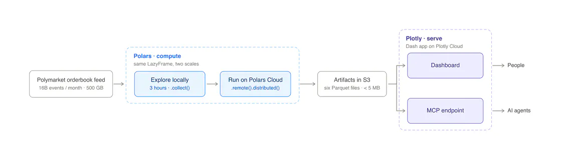
For Plotly Cloud, there's almost nothing to configure. Plotly Cloud provisions the production server, so the app carries no Procfile, no exposed server object, no if "__name__" "__main__" guard. You needn't even declare dependencies — Cloud infers them from your code — though pinning them is worth it for reproducible builds:

# pyproject.toml (optional)
dependencies = [
    "dash[cloud,fastapi]>=4.3.0,<5",   # cloud tooling + FastAPI backend
    "uvicorn[standard]",               # WebSocket-capable server
    "plotly>=6.6,<7",
    "polars>=1.39,<2",
    "boto3",                           # reads artifacts from S3
]

Then publish — two commands from the terminal (or the Cloud UI, or Dash dev tools):

pip install "dash[cloud]"
plotly app publish --name polymarket-analytics

That's the throughline below: each capability is something you'd normally build and run yourself, and on Cloud each is just a setting.

Once the app is published, every remote query also shows up in the Polars Cloud dashboard with its own Query Details view: wall time, rows read, per-stage progress, and a stage graph of how the scans, group-bys, and joins were spread across the cluster. The market profile job below read 24 billion rows across its scans and finished in 2m 51s of wall time, packing 18 minutes of node time into that window. When a job is slower than expected, the query profiler is where you find the bottleneck.

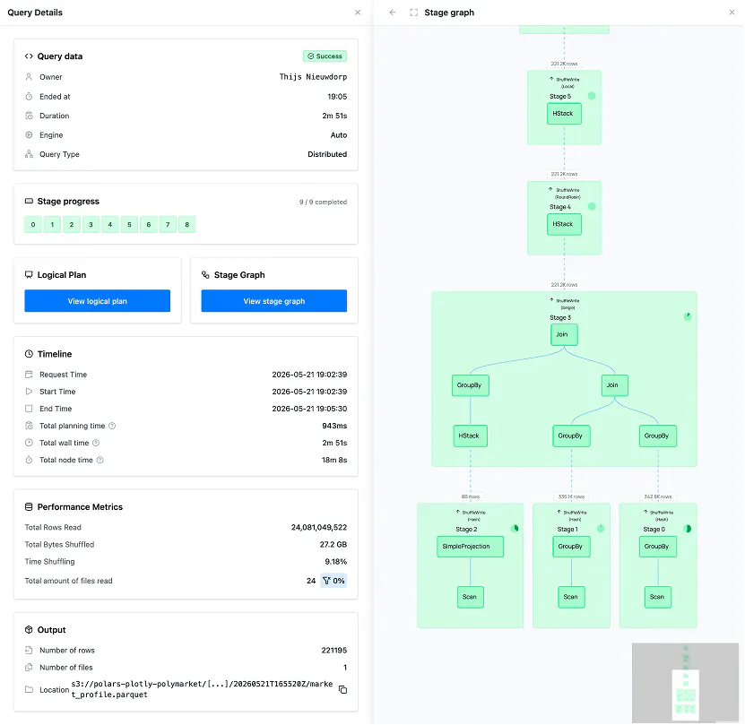
The market profile job in Polars Cloud: 24 billion rows read, nine stages, 2m 51s wall time.

The workflow is not tied to our managed cloud either. Polars Distributed also runs on your own Kubernetes cluster, so the same laptop-to-cluster step works entirely inside your own infrastructure.

Large data, backed by a high-performance store

A data-heavy app on Plotly Cloud rests on one decision: split compute from serve. Do the expensive work once, upstream, and write the results to a store built for fast reads. The Dash app becomes a thin, stateless serving layer that Cloud hosts, connects to your data, and sizes to the working set. Kept Always-On, that layer also acts as a warm in-memory cache in front of the store: repeat reads stay on the box instead of going back to S3, so loads are quick after the first (more below). What the platform handles for that layer:

Managed connectivity. Apps reach external sources (S3, a warehouse, an internal API) over the network, and Cloud publishes stable egress IPs you can allowlist through a firewall. Credentials live in environment variables or come from the app's cloud role, never in code.
A machine sized to the data. Pick a tier matched to the resident working set — no instances to provision or autoscale.
Zero server ops. A click triggers a small, indexed read, not a 500 GB scan — the big computation is paid once per refresh, not once per visitor.

The store is your choice. Here Polars Cloud writes sorted, query-optimized Parquet to S3 (heaviest artifact under 5 MB), but the pattern is identical with a warehouse (Snowflake, BigQuery, ClickHouse), DuckDB over Parquet, or Redis for hot lookups. The app doesn't care which — only that reads are fast and payloads small.

On startup the app reads a small manifest.json to discover which data run is live (the pipeline writes it last, atomically, so the app never reads a half-updated run). Per-market data is fetched on demand and cached, so each market is read at most once:

@lru_cache(maxsize=128)
def query_price_and_spread_data(market_id: str) -> pl.DataFrame:
    return (
        pl.scan_parquet(artifact_url("prices.parquet"), storage_options={"aws_region": AWS_REGION})
        .filter(pl.col("market_id")  market_id)
        .collect()
    )

Because the pipeline sorts prices.parquet by market_id, the reader uses row-group statistics to skip everything that can't match — predicate pushdown against S3, no extra setup. Note that storage_options passes only the region; the S3 client reads credentials from the environment or the app's cloud role, so for a store in the same account you set no secret at all.

A callback fetches that small frame and hands it to a pure figure builder — DataFrame in, figure out — keeping the data and rendering layers separate:

@app.callback(
    Output("price-chart", "figure"),
    Output("spread-chart", "figure"),
    Input("market-dropdown", "value"),
)
def update_selected_market(market_id):
    df = data.query_price_and_spread_data(market_id)   # small read from the store
    label = data.market_name(market_id, 64)
    return figures.price_chart_figure(df, label), figures.spread_chart_figure(df, label)

Why Polars Cloud for the compute half

The store this app reads from is produced by Polars Cloud, a near-perfect fit. The aggregation that runs on one hour locally runs unchanged on a month of 16 billion rows across a cluster, with only the line deciding where execution happens changing — no second framework to drift out of sync with the prototype. It writes Parquet sorted and partitioned exactly how the app reads it, so predicate pushdown does the work. And like Plotly Cloud's metering, it's consumption-based: the heavy compute is a job you run, not infrastructure you operate. The companion Polars post goes deep on that side.

Sizing the machine

The other half of "large data" is the machine. Apps once shared one fixed config; now you choose a tier, from Starter(0.5 vCPU / 1 GB) through Standard (1–2 vCPU) to Performance (4–8 vCPU, 8–16 GB) for heavy computation. Size it to the resident working set, not the source: here the source is 500 GB, but the app holds only a few small artifacts plus cached per-market frames, so it runs comfortably on a modest tier. Scaling that once meant provisioning servers; now it's a connection string and a dropdown.

Controlling Always-On compute

By default, every Cloud app sleeps after 15 minutes idle — the right, free default for an internal dashboard, but a 10-to-30-second wake is unacceptable for a customer-facing one. This app also streams a live order-book replay over a persistent connection (below), which has no business racing an idle timer. Plotly Cloud's app metering gives you direct control, in the app's Compute tab, with two deliberately separate settings:

Sleep is a toggle. Off, the app stays running and the cold start becomes zero.
Machine size is an independent choice, the same tiers as above.

Splitting them means you opt into exactly what you need: a lightweight dashboard turns off Sleep and keeps the smallest machine; a batch-heavy app sizes up without going always-on. This app wants both.

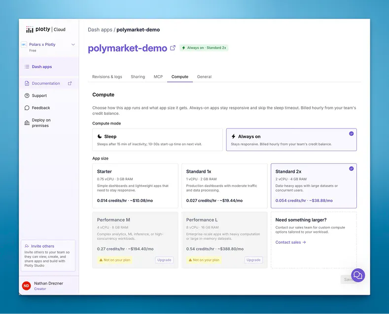
Configuring app size and availability takes a handful of clicks.

Staying awake has a quieter payoff: the app keeps its process, and everything in it. The @lru_cache from earlier survives across requests and users — a market read once stays resident and serves instantly to everyone after — whereas a sleeping app discards that working set on each cold start and rebuilds it from S3. Always-On turns any in-process, ephemeral cache into a genuinely warm one, a useful pattern for read-through layers like this.

Because it's metered, you get cost visibility. Billing is hourly against your team's credit pool — the same credits that power Plotly Studio. Consumption is tracked per app and machine size, so a team sees exactly where its compute spend goes; if the balance runs out, the app reverts to sleep on its own (nothing breaks) and admins get a top-up email. A Standard 1x tier (1 vCPU / 2 GB) meters at about 0.027 credits/hour — running it always-on around the clock is roughly 20 credits a month, and the Compute tab shows the number before you commit. (Rates are set per plan.)

Tip: pair Always-On with any app that holds a persistent connection. Idle-sleep is fundamentally at odds with an open connection, so turn Sleep off and the session stays alive as long as the tab is open. With async callbacks the connections themselves are cheap — each is a coroutine costing kilobytes, not a thread holding ~8 MB — so a modest machine holds many simultaneous sessions. What you size up for is figure-building throughput, not connection slots.

The live replay

The depth chart animates frame-by-frame via a WebSocket callback (Dash 4.2+) — the server pushes frames over a persistent connection instead of the browser polling a dcc.Interval. The replay is a persistent=True callback that runs for the session's life, reading live UI state with ws.get_prop and pushing figures with set_props:

app = dash.Dash(__name__, backend="fastapi", websocket_callbacks=True)


@app.callback(persistent=True)
async def stream_depth_replay():
    ws = ctx.websocket
    while not ws.is_shutdown:
        market_id = await ws.get_prop("market-dropdown", "value")
        if await ws.get_prop("depth-playing", "data") and market_id:
            fig, label = figures.depth_chart_figure(...)
            set_props("depth-chart", {"figure": fig})       # push, don't poll
        await asyncio.sleep(0.6)

Plotly Cloud detects WebSocket callbacks and configures the server for you — no Procfile tuning, no worker class to pick. The only change from a stock Dash app is requesting the FastAPI backend and WebSocket-capable server in dependencies (dash[cloud,fastapi], uvicorn[standard]); Cloud does the rest, and Always-On keeps the connection alive across the session.

Configuring MCP auth

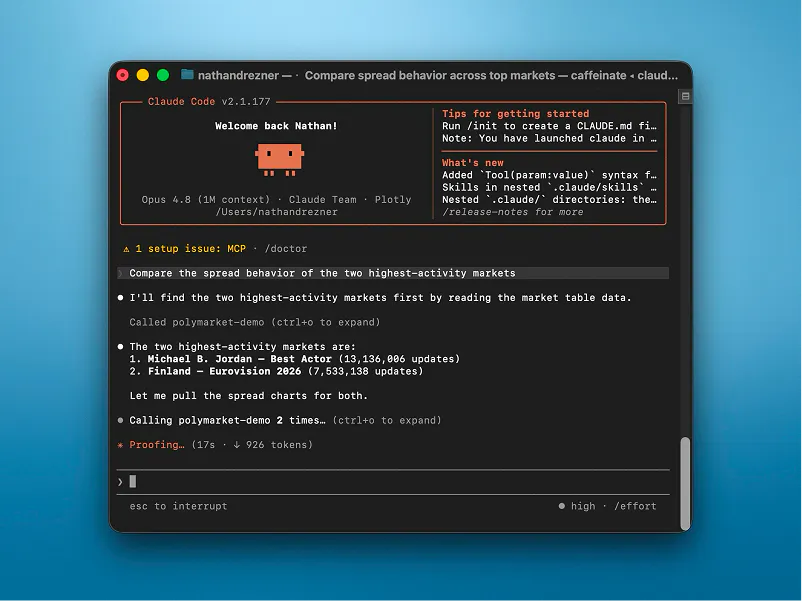
Dash 4.3 lets any app act as a Model Context Protocol (MCP) server: enable it, and an agent like Claude, Cursor, or ChatGPT can connect, discover the app's layout, datasets, and callbacks, and call those callbacks as tools. Instead of answering from general knowledge, the agent queries this app's actual artifacts. Enabling it is one argument, with configure_mcp_server to narrow what the agent sees:

app = dash.Dash(__name__, enable_mcp=True)


configure_mcp_server(
    include_pages=False,              # don't expose the page registry
    expose_callback_docstrings=True,  # hand the agent your callback docstrings
)

A client then points at the app URL plus /_mcp; in Claude Code, one command:

claude mcp add polymarket-analytics --transport http --scope user \
    https://polars-cloud-demo.plotly.app/_mcp

The hard part isn't the protocol — Dash implements that — it's authentication. A private app can't just open an unauthenticated tool endpoint to the internet: the user behind the agent has to sign in, and you have to decide who's allowed. Self-hosting means implementing the full OAuth 2.0 flow yourself; on Dash Enterprise, authenticated MCP isn't supported yet. On Plotly Cloud, there's nothing to implement — the platform handles OAuth using the same access controls as the rest of your app:

Existing sharing settings govern MCP access. A user who can open the app in a browser can connect an agent; one who can't, can't. No API keys, no session tokens, no auth code.
You enable it from the app's MCP tab. Toggle it on (Dash 4.3+) and Cloud surfaces a Connect an AI client dialog; when the client connects, the user signs in with their Plotly Cloud account and the platform runs that sign-in.
Asleep is fine. An MCP request wakes a sleeping app and answers once up, like a browser visit.

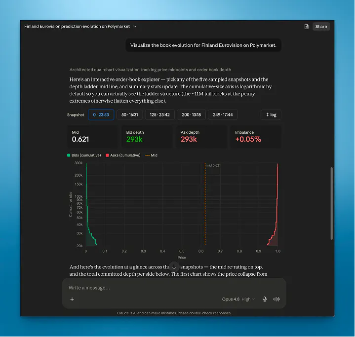
Exploring the data from Polars Cloud using the Dash app as an MCP server connected to Claude Web. The app exposes MCP tools which Claude can use to produce novel insights.

A note on exposure: MCP presents your layout and callbacks — the same view a browser sees, never source code or internal variables. It does surface callback function names, so don't treat a hidden input as access control; enforce permissions explicitly.

Why Plotly Cloud

A general-purpose container host (Render, Heroku, HuggingFace Spaces) or a raw VM can keep a process warm and run a bigger machine. That's where they stop. A data app also needs authentication and collaboration, and you shouldn't have to build either. On Plotly Cloud, apps are private to your team by default and access is a setting, not code — three permission levels (No access, Can view, Can edit) granted to the team, named individuals, or "anyone with the link," with no login page to maintain. Sharing a dashboard with a client is adding them as a Viewer, not standing up separate infrastructure.

That same access model governs your AI agents: the settings that decide who can open the app in a browser also decide who can connect an agent over MCP. One permission list covers humans and agents at once — on a generic platform, MCP access would be a second auth system to keep in sync with the first.

One platform to deploy, scale, and expose

The data work belongs to Polars: decoding and aggregating 16 billion events, the same query local and distributed. Everything downstream is Plotly Cloud, and each piece is a setting rather than a system you operate — a store and a machine tier sized to the working set, Sleep and machine size metered against a shared credit pool, private-by-default sharing with no login code, and MCP exposed under that same access model. Publishing is two commands, and Plotly Cloud is free to start:

pip install "dash[cloud]"
plotly app publish

You're live in minutes. And see the companion Polars post for how the data behind this one is built.