
Chris Parmer
October 23, 2026
Machine Learning Apps in Python with Dash: 3 Real Examples
TL;DR
- Most machine learning tooling is built for training models. The work that comes after, where someone turns a model's output into a decision and keeps an eye on it once it's running, usually happens in slides and spreadsheets.
- A small Dash app, written in Python next to the model, can cover that work. We built three on public data (a bank's call list, an image classifier and a bike-demand forecast), each in 280 to 384 lines of Python.
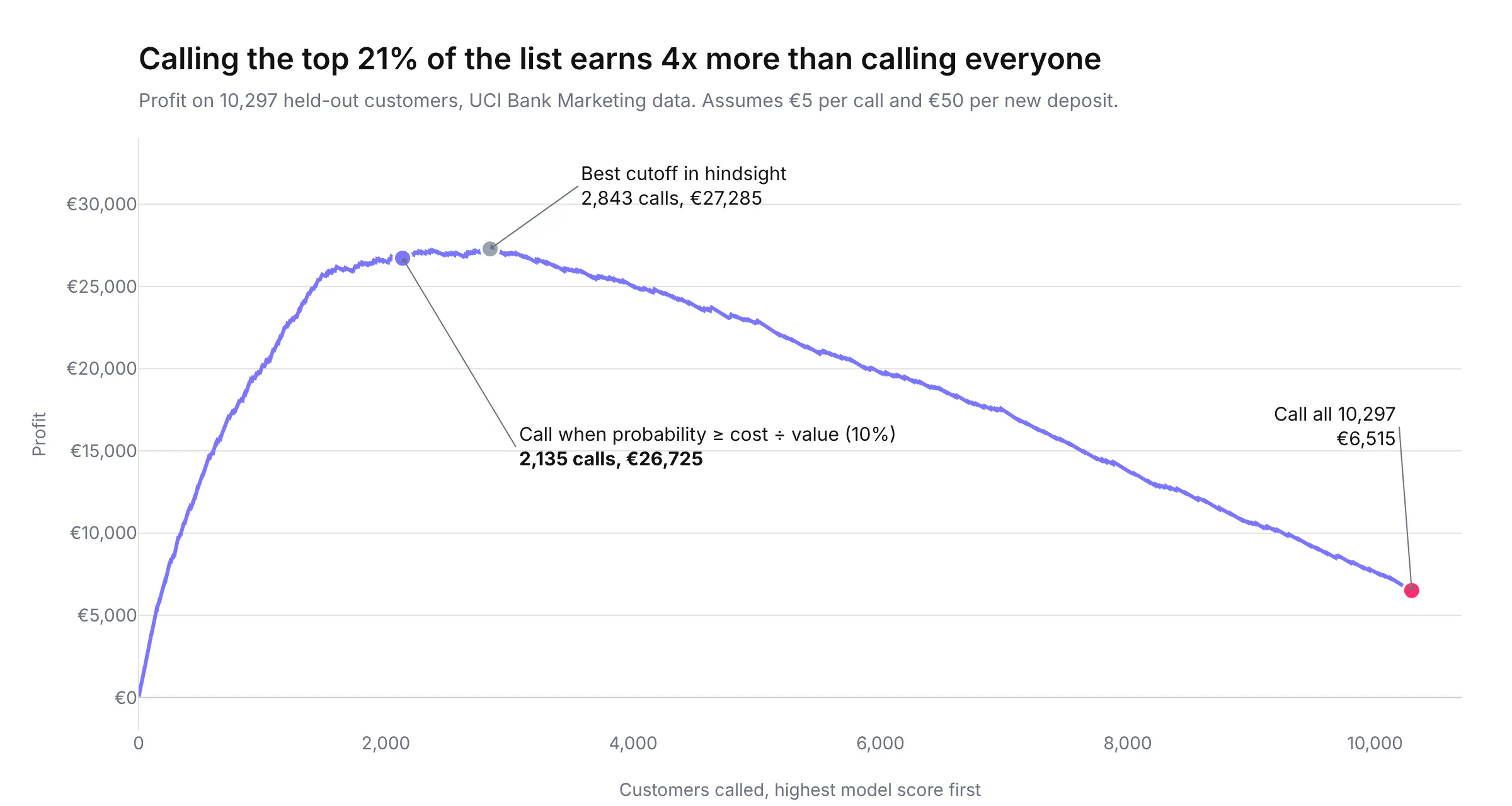
- In each case, looking at the model through an app changed what we concluded about it. The call list earned four times as much as calling everyone at our assumed costs, the classifier's most confident mistakes included mislabeled images, and monthly retraining didn't fix a broken forecast while one new input did.
- Every app also runs as an MCP server, so an AI agent gets the same numbers as the people using the page.
Most machine learning teams are good at training models, and most of the tooling they buy is built for that part: notebooks, experiment trackers, feature stores, training clusters. The trouble starts after the model works. A marketing lead needs to know who to call and what it will earn, not that the AUC is 0.80. A labeling team needs to see the images the model gets wrong, and they don't run notebooks. An operations manager needs to know whether last quarter's forecast can still be trusted. Those answers usually travel as screenshots in a slide deck, which go stale the week after they're made.
A machine learning app is the fix for that gap: a small, purpose-built web app, written in Python next to the model, that shows the model's output to the people who act on it. Coding agents have made these apps much cheaper to build than they were two years ago. This post walks through three of them, each solving a problem that ML teams run into in production, with real public data, the numbers they produce and the code. It's written for two readers: data leaders deciding where apps like these fit in their ML strategy, and ML engineers who want to build one.
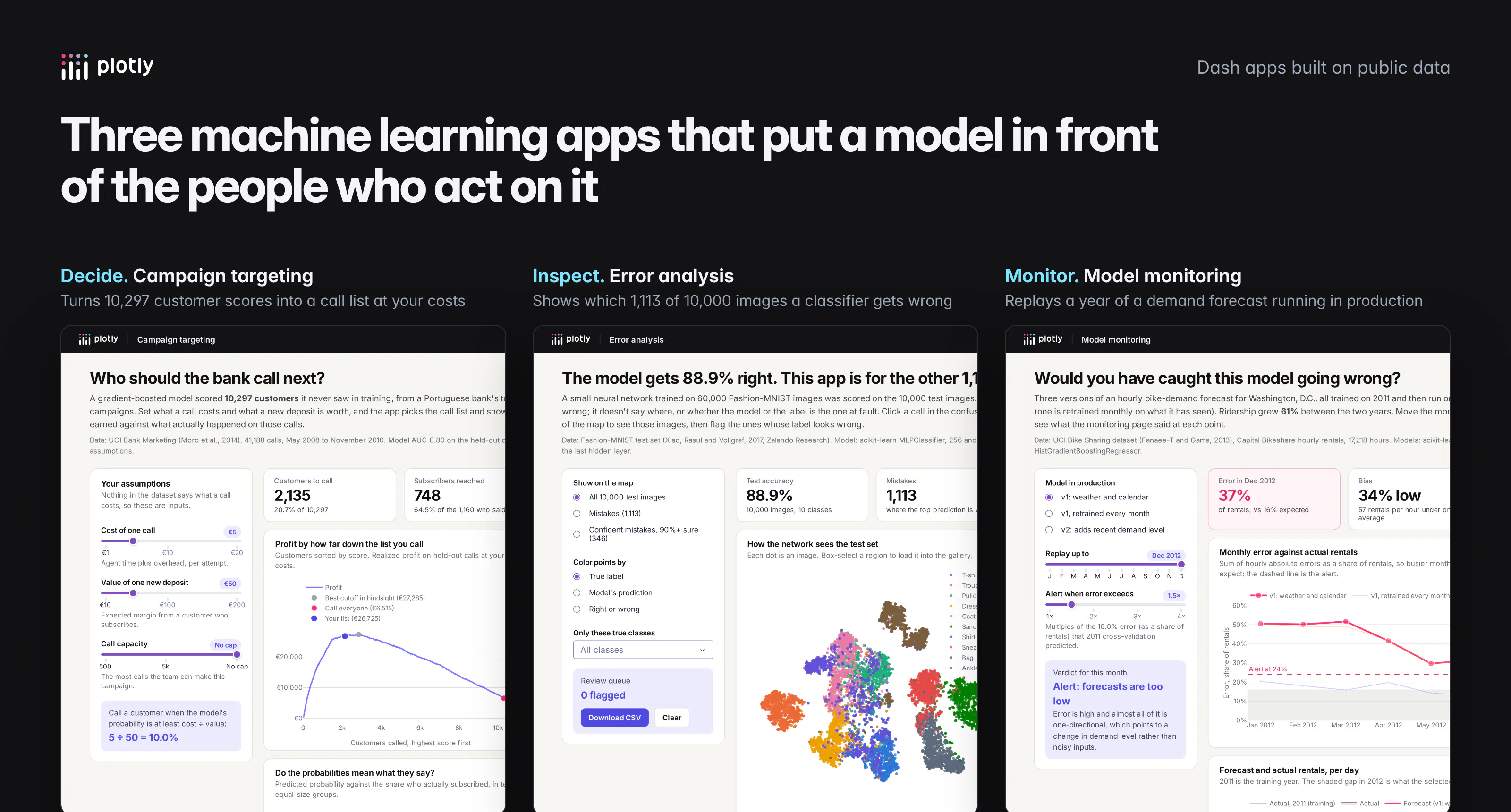
The three apps
App
Data
What it answers
Campaign targeting
UCI Bank Marketing, 41,188 phone calls (2008-2010)
Who should we call, and what will it earn?
Error analysis
Fashion-MNIST, 10,000 test images
Where is the model wrong, and is it the model or the label?
Model monitoring
UCI Bike Sharing, 17,218 hours of rentals (2011-2012)
Is the model in production still right, and if not, why?
All three use scikit-learn models trained offline. The training scripts write the model's predictions to a file, and the app reads that file when it starts, so every interaction in the browser is a fast pandas operation instead of a model call. That split, heavy work in a scheduled job and light work in the app, is the pattern we'd use for most production ML apps.
Where does Dash fit in a machine learning stack?
Dash is Plotly's open-source Python framework for data apps. It doesn't train models, store features or replace your experiment tracker. It covers the steps where someone outside the ML team has to understand a model's output and do something with it, which in most companies are the steps with no tooling at all.
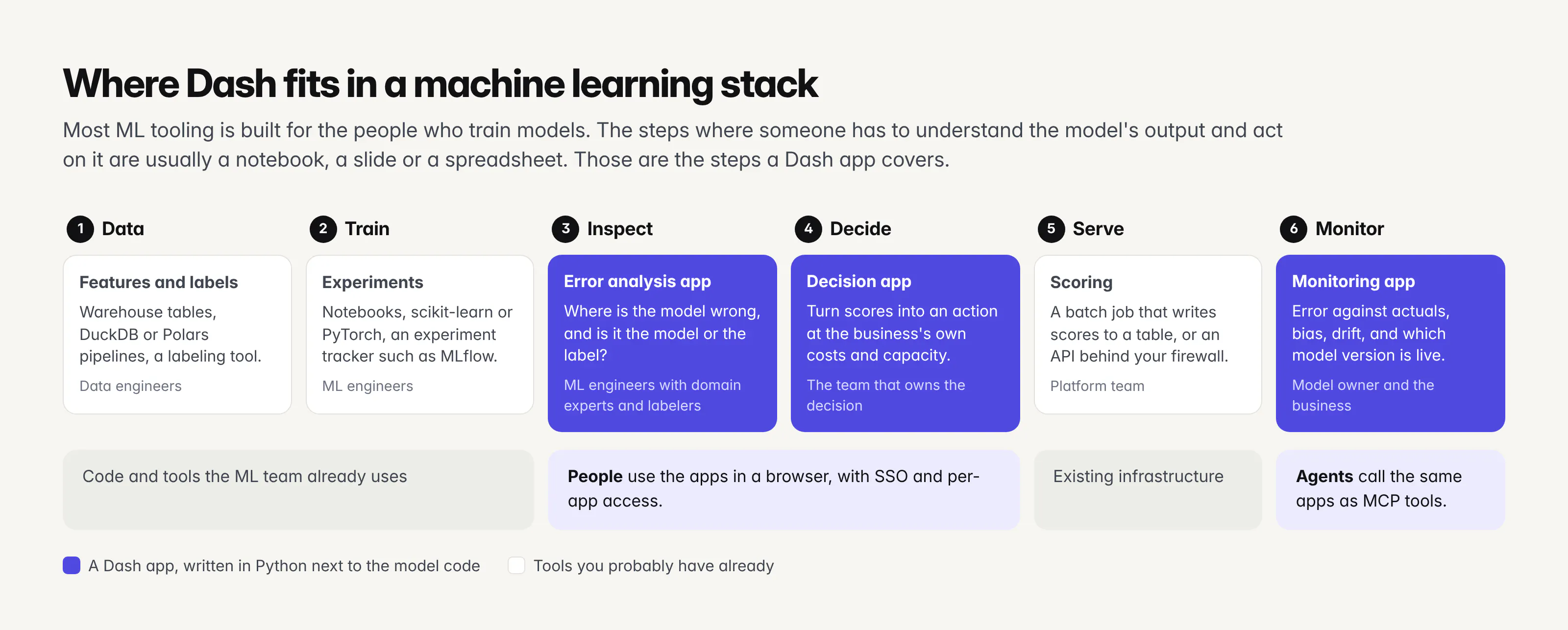
For a data leader, the useful way to think about it is that a model isn't finished when it scores well. It's finished when the people who own the decision can see what it recommends at their own costs, check where it's wrong, and tell when it stops working. Each of those is a small app with a named owner, and because the app is Python code in the same repository as the model, the ML team can build and change it without handing a spec to a front-end team. In practice, the person who trained the model asks a coding agent like Claude Code or Codex for the app, reads the diff and ships it.
For an ML engineer, the appeal is that everything stays in Python. The app imports the same pandas DataFrames and scikit-learn objects as the training code, callbacks are plain functions, and Plotly's charts cover the plots ML work needs (calibration curves, confusion matrices, 10,000-point embeddings with WebGL) without writing JavaScript.
Example 1: How do you turn model scores into a business decision?
The UCI Bank Marketing dataset records 41,188 phone calls a Portuguese bank made between May 2008 and November 2010 to sell term deposits. 11.3% of the people called said yes. We trained a gradient-boosted classifier (scikit-learn's HistGradientBoostingClassifier) on 75% of the calls and kept 10,297 calls aside, so we can see what the model's choices would have earned against what actually happened.
The dataset's documentation warns that the call duration column predicts the outcome almost perfectly, because a call that ends after five seconds didn't sell anything, and that nobody knows the duration before dialing. With it, our model's AUC was 0.95. Without it, 0.80. We dropped it, and 0.80 is the honest number. Leaks like this are common in business data, and they're much easier to spot when someone looks at what the model depends on, which is one of the four charts in the app.
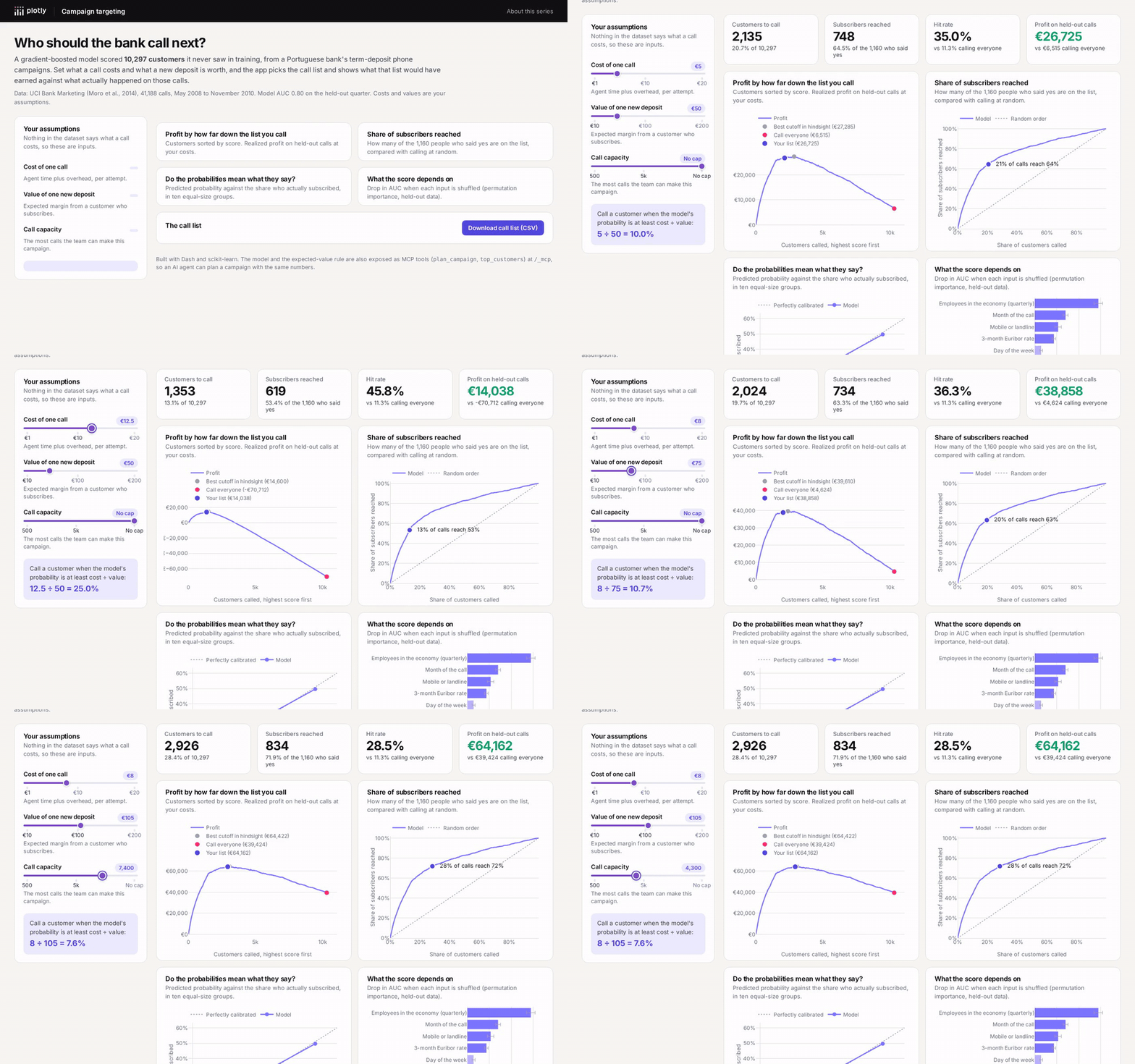
An AUC of 0.80 doesn't tell anyone who to call. The decision needs two more numbers the dataset doesn't have: what a call costs and what a new deposit is worth. The app makes those inputs, with sliders. Given them, decision theory gives a simple rule: call a customer when their predicted probability is at least cost ÷ value. At €5 per call and €50 per deposit, that threshold is 10%.
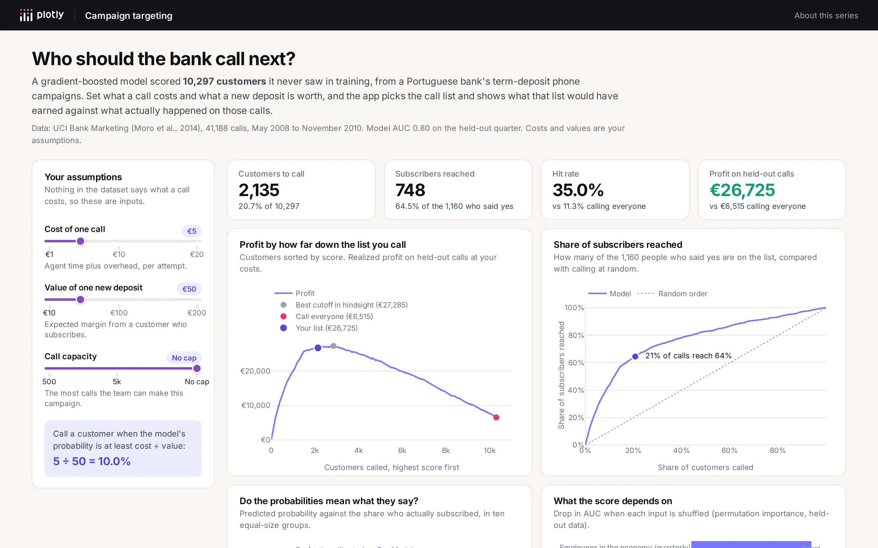
On the held-out calls, at those costs, the rule says to call 2,135 customers (20.7% of the list). That list reaches 748 of the 1,160 people who subscribed, a 35.0% hit rate against 11.3% for calling everyone, and earns €26,725 against €6,515. The best cutoff we could have picked with hindsight, knowing the outcomes, earns €27,285, so the rule gets 98% of the way there without seeing a single outcome. At €10 per call, calling everyone would lose €44,970 while the rule still earns €18,140.
The rule only works if a 10% score means a 10% chance, so the app shows a calibration chart next to the profit curve. This model is close: the top tenth of customers averages a 51.0% predicted probability and 49.6% of them subscribed. If the curve bent away from the diagonal, the fix would be to calibrate the model (scikit-learn's CalibratedClassifierCV), and the app is where you'd notice.
The app also lists the customers to call in a sortable table and downloads the full list as a CSV, which is what the call center actually needs. The whole interaction runs on a precomputed table of 10,297 scores, so the callback behind the sliders takes about 20 milliseconds on our test machine to recompute the numbers, the charts and the call list.
Example 2: How do you find out where a classifier is wrong?
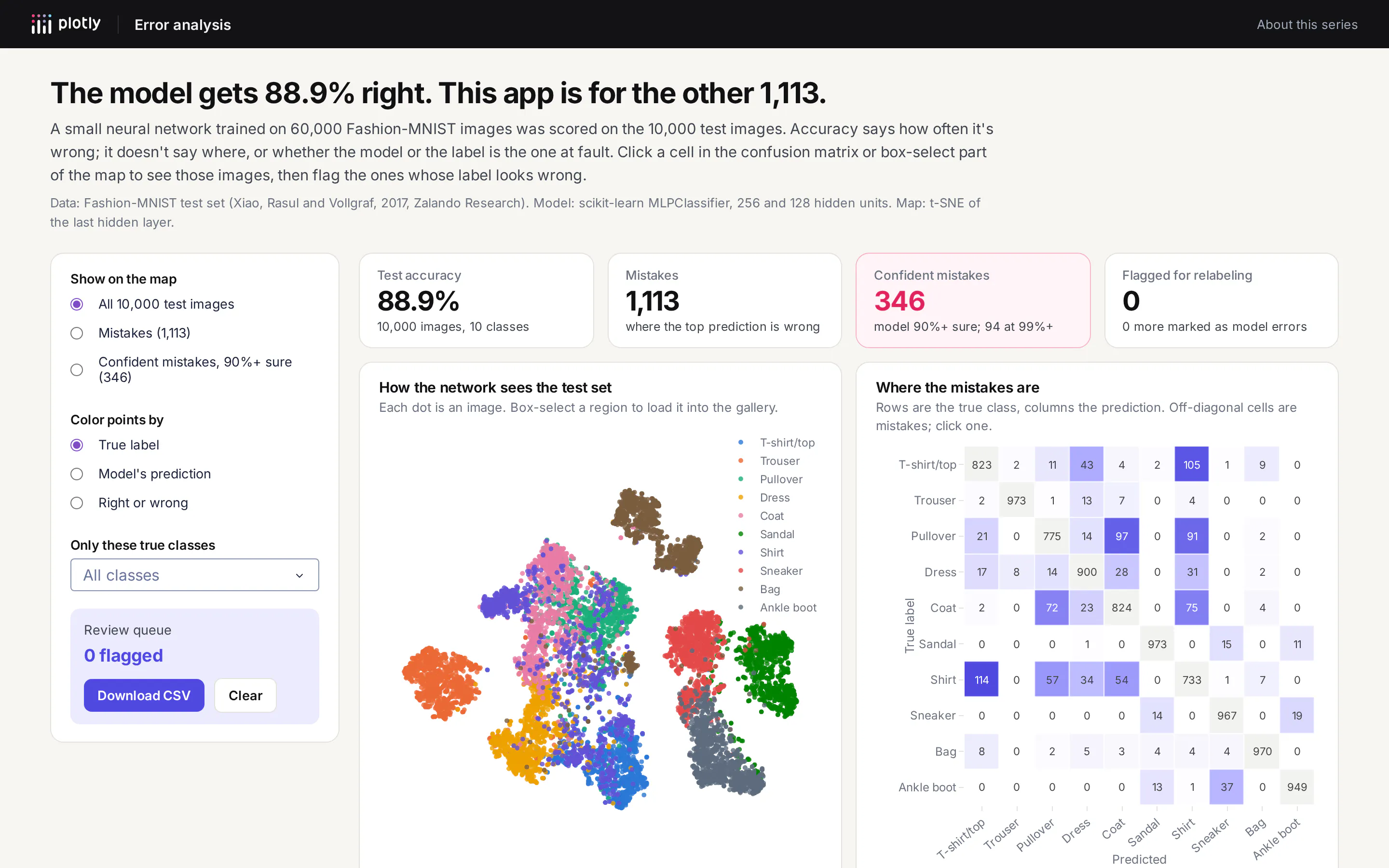
Fashion-MNIST is Zalando Research's set of 70,000 small grayscale photos of clothing in ten classes. We trained a two-layer neural network (scikit-learn's MLPClassifier, 256 and 128 hidden units) on the 60,000 training images. It gets 88.9% of the 10,000 test images right.
That accuracy number hides almost everything useful. The confusion matrix in the app shows the 1,113 mistakes are not spread evenly: shirts, T-shirts, pullovers and coats account for most of them, with 114 shirts called T-shirts and 105 T-shirts called shirts. Shirt is the worst class at 73.3% accuracy, while trousers and bags are both at 97% or better. The map next to it is a t-SNE projection of the network's last hidden layer, and it shows the same thing visually: shoes, bags and trousers form clean islands, while the upper-body clothing overlaps in one cloud.
The most useful view is the gallery of the model's most confident mistakes. The model made 346 mistakes while at least 90% sure, and 94 while more than 99% sure. When we went through those 94, some were plainly mislabeled: a lace-up heeled boot labeled "Sandal", an open-toe heel labeled "Ankle boot", a long sleeveless dress labeled "T-shirt/top". Many sat on the blurry border between shirt and T-shirt, where reasonable people would disagree. And some were the model being confidently wrong, like a T-shirt it called a bag. A metric can't separate those three cases, but a person looking at the picture can in about a second.
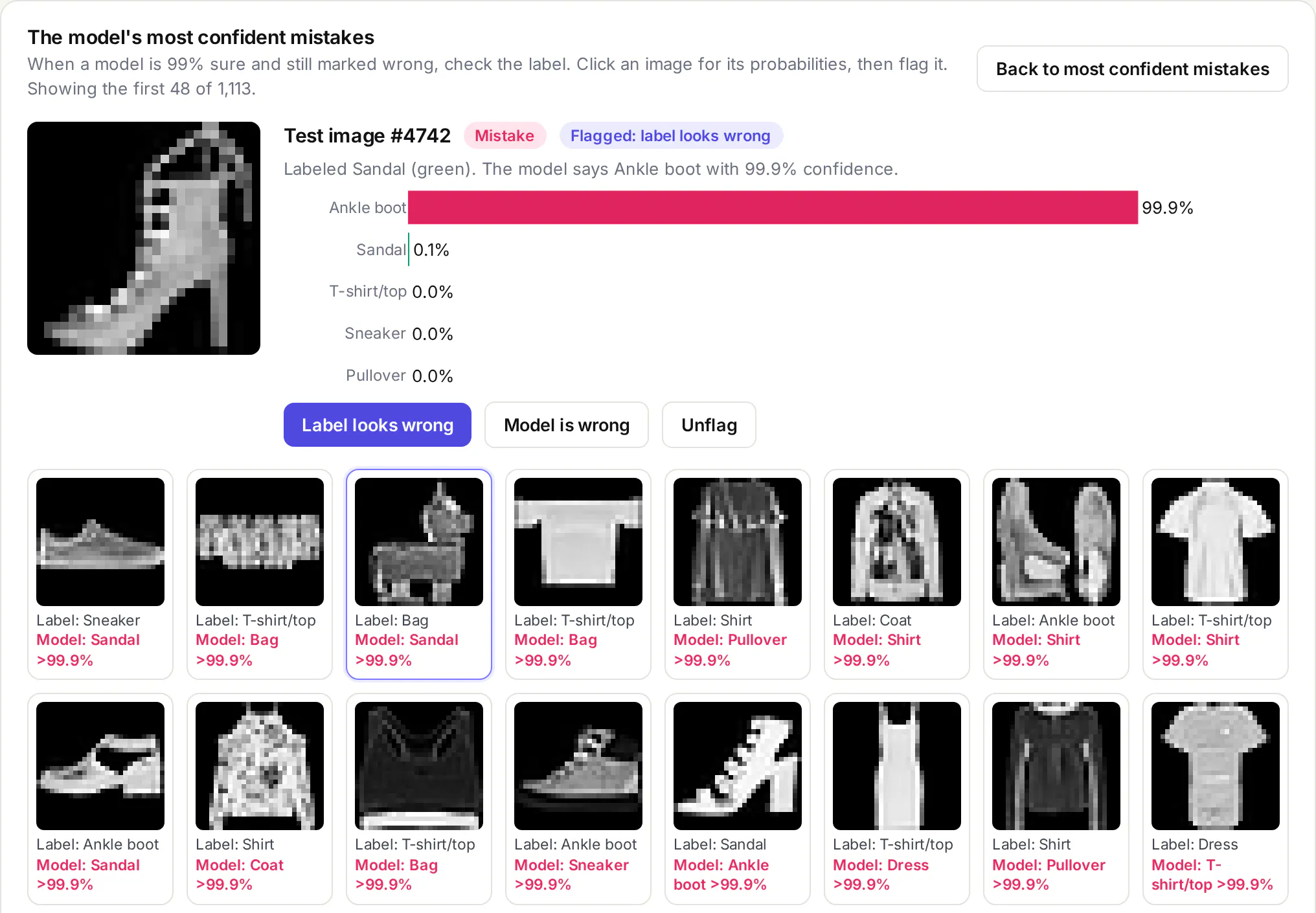
So the app lets you flag each image as "label looks wrong" or "model is wrong", keeps the flags in your browser, and downloads them as a CSV to send back to whoever owns the labels. Clicking any cell of the confusion matrix loads those images, and box-selecting part of the map loads that region, which is how you find a cluster of near-duplicates or a class that's really two classes.
This is the app where Dash pays off most for engineers, because the people who can judge a mislabeled X-ray, a misrouted support ticket or a false fraud alert are domain experts, not the people who trained the model. Giving them a page instead of a notebook is the difference between getting their review and not.
Example 3: How do you monitor a machine learning model in production?
The UCI Bike Sharing dataset has hourly rental counts from Capital Bikeshare in Washington, D.C., for 2011 and 2012, with the weather for each hour. We trained models on 2011 only and then ran them on 2012 without letting them see it, which is what happens to a model after it's deployed. Ridership grew 61% between the two years, from 145 to 235 rentals an hour on average.
We tested three versions:
- v1 predicts hourly rentals from the hour, the type of day and the weather.
- v1, retrained every month is the same model, refit at the start of each 2012 month on everything seen so far, which is what many teams schedule when they worry about drift.
- v2 adds one input, the average number of rentals per hour over the previous seven days, and predicts demand relative to it.
To know what "wrong" means, the monitor needs an expected error. Cross-validation on 2011, holding out whole weeks, said v1 should be off by about 16.0% of rentals. Because ridership grew, the monitor measures error as a share of rentals rather than in rentals per hour, otherwise a busier year looks worse even when the model is just as good.
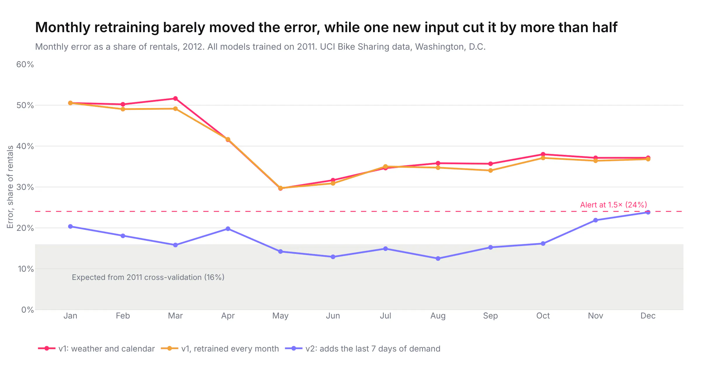
v1 was off by 51% of rentals in January 2012, its first month live, and 38% across the year, almost all of it in one direction: it under-forecast by 86 rentals an hour on average. An alert set at 1.5 times the expected error fires in all 12 months. Retraining every month barely helped (37.5% for the year), because nothing in the inputs tells the model that ridership is growing, so more data of the same kind can't fix it. v2, which sees recent demand, was off by 16.5% across 2012, almost exactly what 2011 testing predicted, and it never crossed the alert line, although December came close at 23.8% against a 24.0% limit.
The monitor also tracks input drift, the population stability index (PSI) of each weather input against the same month a year earlier, and this turned out to be the less useful signal. Weather drift checks fired 10 times out of 48 in 2012 (January 2012 averaged about 11 °C against 7 °C a year earlier, for example), and they fire the same way whichever model is running, because they only look at the inputs. They didn't tell us v1 was broken or that v2 was fine. Error against actual outcomes did.
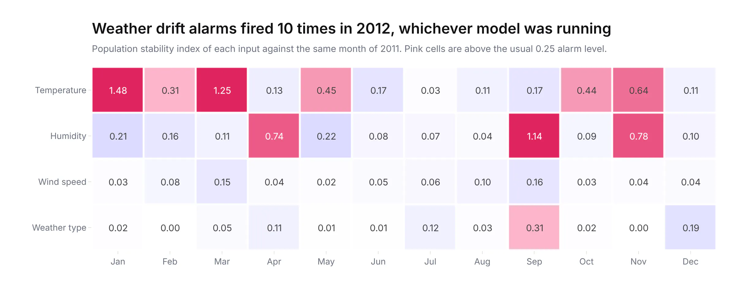
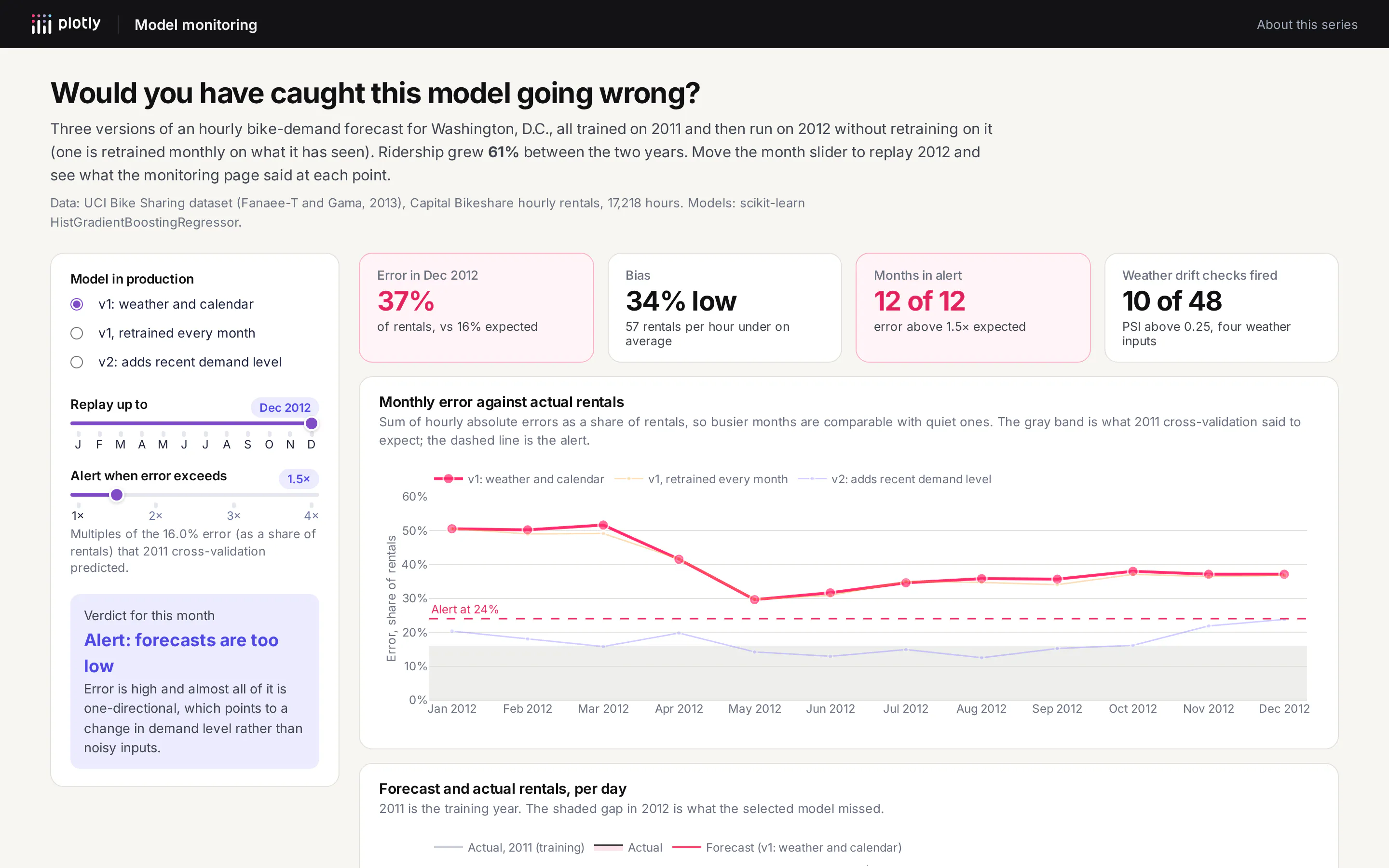
For data leaders, this is the example to take to a planning meeting. Monitoring that only watches inputs is cheap to set up and generates a lot of alerts, but it can't tell you whether the model is right. Monitoring against outcomes needs the actual values to come back (sales, rentals, defaults), which means someone has to plan for that data when the model is built. And the fix for a broken model is often a better feature rather than a retraining schedule, which is a decision that needs a person looking at the right chart.
How do AI agents use the same model?
Since Dash 4.3, any Dash app can also be an MCP server, the protocol that AI agents like Claude, ChatGPT and Cursor use to call tools. On Plotly Cloud, the app's sharing settings decide who can connect an agent to it, so there are no extra keys to manage. We turned it on in all three apps and exposed a few plain Python functions as tools with the mcp_enabled decorator:
from dash import Dashfrom dash.mcp import configure_mcp_server, mcp_enabledapp = Dash(__name__, enable_mcp=True)configure_mcp_server(include_callbacks=False) # expose only the tools below@mcp_enabled(name="plan_campaign", expose_docstring=True)def plan_campaign(cost_per_call: float = 5.0, value_per_subscription: float = 50.0, max_calls: int = 0) -> dict:"""Plan a phone campaign from the term-deposit model's scores on 10,297 held-out bank customers.Calls a customer when their probability of subscribing is at least cost_per_call / value_per_subscription."""return plan(cost_per_call, value_per_subscription, max_calls or None)
When an agent calls plan_campaign with €5 and €50, it gets back the same 2,135 calls, 748 subscribers and €26,725 the page shows, because both run the same function. The error app exposes top_confusions, class_report and confident_mistakes, so an agent can pull a relabeling list, and the monitor exposes model_health and compare_models, so an agent can check on the forecast every Monday without anyone opening the page.
This matters for ML strategy because it gives one place where a model's business logic lives. The threshold rule, the definition of "error" and the alert level are reviewed Python code in the app's repository, and both people and agents get answers from it, rather than each chatbot conversation re-deriving them slightly differently.
How to build a machine learning app like this
In Python
Here is the smallest useful version of the campaign app. It downloads the data, trains the model and serves the decision rule with two sliders, in 51 lines. Run pip install dash scikit-learn pandas requests, then python minimal_app.py, and open http://127.0.0.1:8050.
import ioimport zipfileimport numpy as npimport pandas as pdimport plotly.express as pximport requestsfrom dash import Dash, Input, Output, callback, dcc, htmlfrom sklearn.ensemble import HistGradientBoostingClassifierfrom sklearn.model_selection import train_test_split# UCI Bank Marketing: 41,188 phone calls. "duration" is dropped because it's only known after the call.url = "https://archive.ics.uci.edu/static/public/222/bank+marketing.zip"outer = zipfile.ZipFile(io.BytesIO(requests.get(url, timeout=60).content))inner = zipfile.ZipFile(io.BytesIO(outer.read("bank-additional.zip")))df = pd.read_csv(inner.open("bank-additional/bank-additional-full.csv"), sep=";").drop(columns="duration")y = (df.pop("y") == "yes").astype(int)for c in df.select_dtypes(exclude="number"):df[c] = df[c].astype("category")X_train, X_test, y_train, y_test = train_test_split(df, y, test_size=0.25, stratify=y, random_state=7)model = HistGradientBoostingClassifier(categorical_features="from_dtype", random_state=7).fit(X_train, y_train)scores = pd.DataFrame({"p": model.predict_proba(X_test)[:, 1], "y": y_test.to_numpy()}).sort_values("p", ascending=False)app = Dash(__name__)app.layout = html.Div([html.H2("Who should we call?"),html.Label("Cost of a call (€)"), dcc.Slider(1, 20, 0.5, value=5, id="cost", marks=None, tooltip={"always_visible": True}),html.Label("Value of a new deposit (€)"), dcc.Slider(10, 200, 5, value=50, id="value", marks=None, tooltip={"always_visible": True}),html.H3(id="summary"),dcc.Graph(id="profit"),], style={"maxWidth": 900, "margin": "auto", "fontFamily": "Inter, sans-serif"})@callback(Output("summary", "children"), Output("profit", "figure"), Input("cost", "value"), Input("value", "value"))def update(cost, value):call = scores.p >= cost / value # the expected-value ruleprofit = np.cumsum(scores.y) * value - np.arange(1, len(scores) + 1) * costfig = px.line(x=np.arange(1, len(scores) + 1), y=profit, labels={"x": "Customers called", "y": "Profit (€)"})fig.add_vline(x=call.sum(), line_dash="dot")hits = scores.y[call].sum()return f"Call {call.sum():,} customers, reach {hits:,} subscribers, earn €{hits * value - call.sum() * cost:,.0f}", figif __name__ == "__main__":app.run(debug=True)
For a real app, move the training into its own script that writes scores to a file (or a table) on a schedule, and have the app read that file. The full versions of all three apps, with their training scripts, follow that layout. To publish one on Plotly Cloud, run plotly app publish from the app's folder.
With Plotly Studio
Plotly Studio builds a Dash app from a dataset and a description. Load a CSV of model scores and outcomes (one row per customer, with a score and a subscribed column) and ask:
Build a campaign planning app from these model scores. Add sliders for the cost of a call (1 to 20 euros) and the value of a new subscriber (10 to 200 euros). Call everyone whose score is at least cost divided by value. Show how many customers that is, how many actual subscribers it reaches, the hit rate and the profit, compared with calling everyone. Add a chart of profit against the number of customers called, highest score first, and a calibration chart of average score against actual subscription rate in ten equal-size groups.
With a coding agent
In Claude Code, Codex or Copilot, from a repository that has your model's training code:
Write a Dash app that monitors this forecasting model in production. Read predictions and actuals from predictions.parquet (columns: timestamp, model_version, predicted, actual). Show monthly error as a share of actuals for each model version against the error we measured in cross-validation (put that number in a constant), with an alert line at 1.5 times it, and a chart of daily predicted against actual. Add the population stability index of each input feature against the same month a year earlier as a heatmap. Expose a model_health(month, model_version) function as an MCP tool with Dash's mcp_enabled decorator. Use Plotly's default template, run the app and check every chart renders before you finish.
Summary
The three apps cover the parts of a model's life that usually live in slides: turning a score into a decision at the business's own costs, finding out where and why the model is wrong, and noticing when it stops working in production. Each one changed what we concluded from the same model. A 0.80 AUC became a call list worth four times calling everyone, an 88.9% accuracy became a list of mislabeled images, and a forecast that looked fine on its inputs turned out to be 38% off until one new feature brought it back to 16.5%. Because they're Dash apps, they're plain Python next to the model code, and with MCP turned on, the same functions answer an agent's questions too. If your data can't leave your network, the same apps run on Dash Enterprise in your own cluster, with SSO and per-app access.