How to graph ZIP codes in Python: heat maps, bubble maps, and charts

TL;DR

• There are three common ways to graph ZIP code data: a heat map that colors each ZIP code's area, a bubble map with one dot per ZIP code, and a plain chart that treats ZIP codes as categories. Each one is a few lines of Python with Plotly, and the code below makes all three from one dataset.
• The maps need ZIP code shapes, which is the hard part, because ZIP codes are mail routes rather than areas and had no official shape from 1963 until USPS started selling one in September 2026. The Census Bureau's ZIP Code Tabulation Areas (ZCTAs) are a free stand-in: 33,791 polygons in one 529 MB download.
• Free shapes are close enough for most graphs. When we put 77,208 bank branches into them, 96.8% landed in the ZCTA matching the ZIP code on their address.
• Five examples on public data show what ZIP code maps can do in finance, energy, and pharma: income per tax return, clean energy credits, electricity rates, clinical trial sites, and bank branches per return.
• The details that trip people up are leading zeros, ZIP codes with no shape, ZIP codes that cross county lines (30.1% of ZCTAs do), suppressed small counts, HIPAA's three-digit rule for patient data, and big rural ZIP codes that dominate the map. A dos and don'ts checklist sums them up.

Almost every dataset that touches people arrives keyed by ZIP code: insurance policies, loan applications, prescription claims, clinical trial sites, and utility accounts. The first thing most people want to do with it is graph it, usually on a map, and Google's suggestions for "plot ZIP codes on a map" and "ZIP code heat map" are mostly Excel, Power BI, Tableau, and free generators. Those can draw one, but the graph then lives in a workbook or a BI dashboard, apart from the code and data behind the rest of your analysis.

In Python, each graph is a few lines of code. The only part where people get stuck is finding shapes for the ZIP codes. This post uses one real dataset, every FDIC-insured bank branch in the Houston area, to show three ways to graph ZIP codes with Plotly: a heat map, a bubble map, and a bar chart. It also covers a short history of how ZIP codes got their shapes, where to get those shapes for free, five more examples from finance, energy, and pharma, the details that make ZIP code graphs wrong, and how much accuracy you give up with free shapes compared with the official USPS boundaries.

What you need to graph ZIP codes

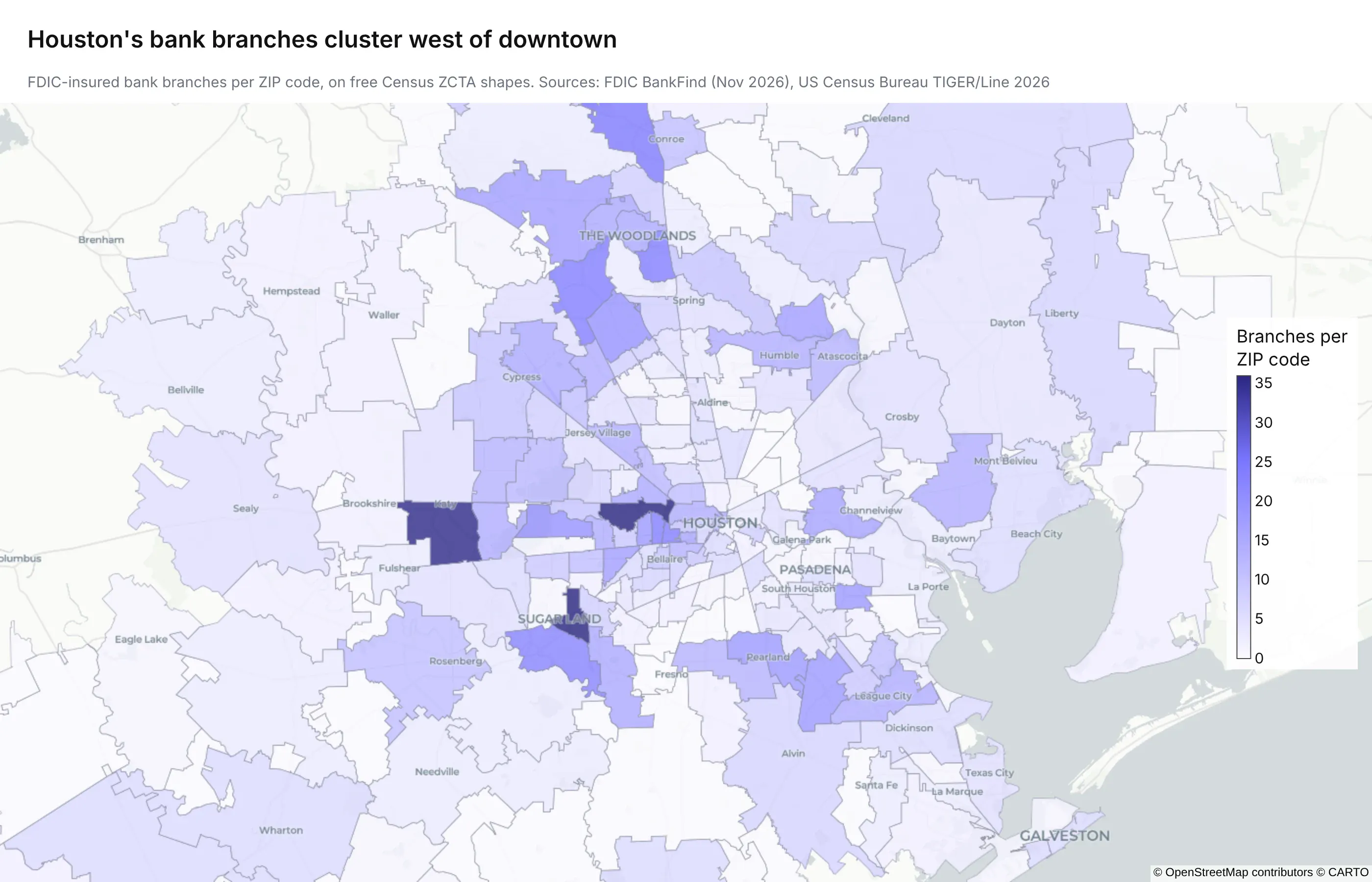
The heat map above counts bank branches across 282 ZIP codes in the Houston area, and it shows something a table wouldn't: the branches cluster west of downtown, in Memorial, Sugar Land, and Katy, rather than in the downtown ZIP code 77002.

To draw a map like it you need two things:

• Your data, with a five-digit ZIP code column and a number per ZIP code (a count, a sum, or a rate).
• A shape for each ZIP code, usually a shapefile or GeoJSON file with one polygon per ZIP code.

The second one is less simple than it sounds, because ZIP codes aren't really areas. A ZIP code is a set of USPS delivery routes, drawn up so the right letter ends up on the right truck. Some ZIP codes belong to a single office tower, some cover only PO boxes, and a few follow a rural road across a state line. Any ZIP code shapefile is someone's best attempt at drawing the area those routes serve. (A bar chart or table doesn't need shapes at all, only the ZIP codes as text.)

A short history of ZIP codes and their shapes

ZIP codes were built for sorting mail, and the shapes came decades later, which explains most of the strange things in this post.

• 1943: postal zones. The Post Office Department gave large cities one- or two-digit delivery zones, as in "Chicago 14, Illinois".
• 1963: the ZIP code. On July 1, 1963, the Post Office introduced the five-digit Zone Improvement Plan (ZIP) code. The first digit is a group of states, from 0 in the Northeast to 9 on the West Coast, and the first three digits name a sectional center facility, the mail processing plant that serves the area. That's why three-digit ZIP codes still make a useful regional grouping.
• 1983: ZIP+4. USPS added four more digits that narrow a ZIP code down to a block face, a building, or a bank of mailboxes. They were designed for sorting machines, and USPS doesn't publish shapes for them.
• 2000: ZCTAs. For the 2000 Census, the Census Bureau started publishing ZIP Code Tabulation Areas, polygons built from census blocks, so that census data could be reported by something close to ZIP code. They're redrawn each decade, and the current set dates from 2020.
• 2026: official USPS polygons. In September 2026 USPS started selling ZIP Code Boundaries built from its own delivery points, updated quarterly.

For most of their history, then, ZIP codes had no official shape at all. Every ZIP code map made between 1963 and 2026 used someone's reconstruction of one, and most still do.

Where to get free ZIP code shapes

There are three common sources, and they trade cost against accuracy and freshness.

For most graphs, use the Census ZCTAs. A ZIP Code Tabulation Area (ZCTA) is the Census Bureau's approximation of a ZIP code's area: the Bureau assigns each census block to the ZIP code most of its addresses use, and merges blocks with the same ZIP code into a polygon. Because ZCTAs are built from census blocks, Census tables (population, income, housing, and health insurance coverage) are also published by ZCTA, which is what you need to turn counts into rates.

The USPS product is new. In September 2026 USPS started selling its own ZIP Code Boundaries, built from residential delivery points and updated every quarter, at the prices in the table (from the USPS order form). It's the better choice when you need ZIP codes created since 2020 or exact edges, and the section on accuracy below compares the two.

How to make a ZIP code heat map in Python

A ZIP code heat map is a choropleth map: each ZIP code is drawn as a shape and filled with a color that stands for a number. This is the code behind the Houston map. It downloads every FDIC-insured bank branch in Texas from the Federal Deposit Insurance Corporation's (FDIC) public BankFind API, counts branches per ZIP code, joins the counts to the Census ZCTA shapes with geopandas, and draws the map with Plotly. Swap step 1 for your own dataframe of ZIP codes and values.

A few notes on adapting it:

• Read ZIP codes as strings. dtype={"ZIP": str} and zfill(5) keep the leading zero in ZIP codes like 02139. Read as numbers, every ZIP code that starts with a zero (New England, New Jersey, and Puerto Rico) fails to join without any error.
• Filter before you plot. All 33,791 polygons at full detail make a very large figure. Filter to your region, or simplify the shapes for a national map (simplify(0.004) in degrees is invisible at country zoom).
• Hover and style. hover_name and hover_data control the tooltip, and the Plotly docs on tile choropleth maps cover color scales, base maps, and outlines.

To put it in front of your team, wrap the figure in a Dash app with a dropdown for the metric or the region, and deploy it to Plotly Cloud or Dash Enterprise.

How to plot ZIP codes on a map as points

A bubble map draws one dot per ZIP code and sizes it by your value. It's the better choice when a few large rural ZIP codes would otherwise dominate a heat map, since every ZIP code gets a dot of the same scale whatever its area. Continuing from the code above, take a point inside each ZCTA and pass it to px.scatter_map:

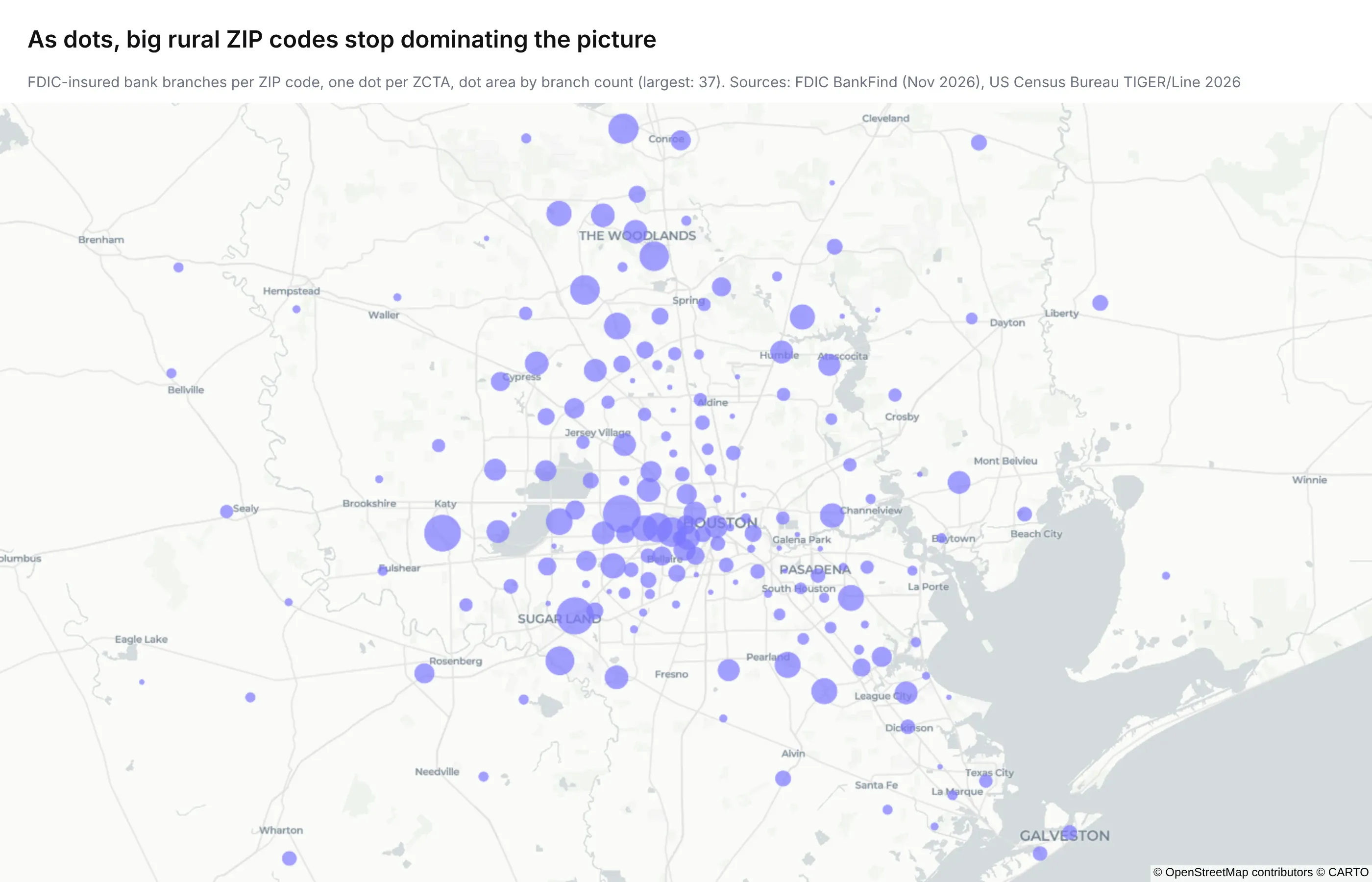
representative_point() is used instead of the centroid because it's always inside the shape, which matters for ZIP codes shaped like a crescent or a ring. The to_crs(2278) step does the geometry in a projected coordinate system (Texas South Central, in feet) so the points are placed accurately.

If you have coordinates and need ZIP codes, run a spatial join. This tags two Houston locations with the ZCTA they fall in:

How to chart ZIP codes without a map

Not every ZIP code graph needs to be a map. When the question is "which ZIP codes have the most", a sorted bar chart answers it faster, and it doesn't need any shapes:

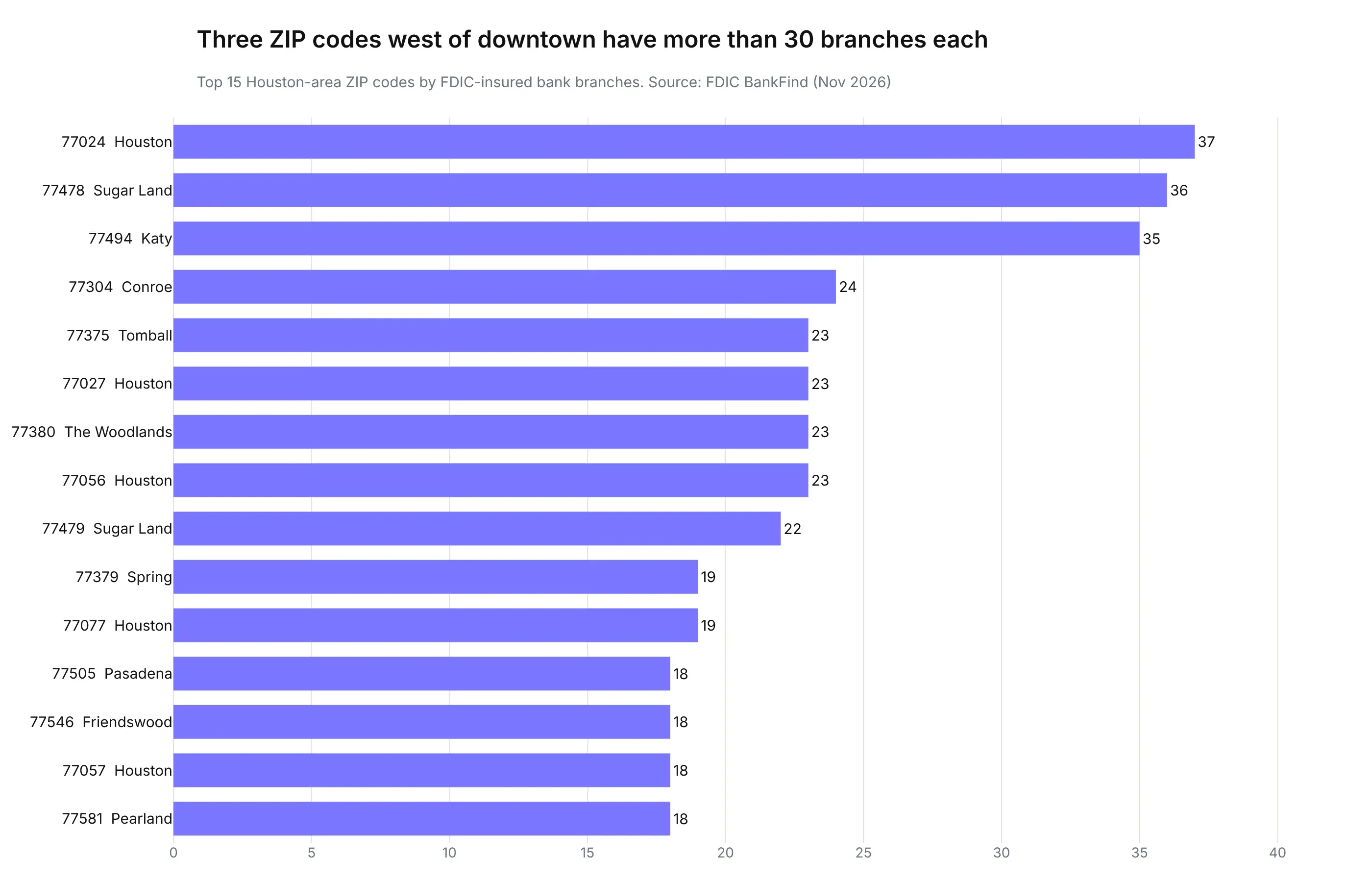
The important line is type="category". Without it, Plotly sees five-digit numbers and draws a numeric axis, with each bar placed at its ZIP code's value instead of in a sorted list. The same goes for any chart with ZIP codes on an axis or in a legend: keep them as text from the moment you read the file. To compare regions rather than single ZIP codes, group by the first three digits (zip.str[:3]), which is how USPS groups ZIP codes for its sectional center facilities.

Five examples of graphing ZIP codes with real data

The Houston maps above use one dataset. These five use others, from the industries where ZIP code data shows up most: finance, energy, and pharma. Each one is a single Plotly figure on the free ZCTA shapes (or three-digit ZIP areas built from them), and each one shows a different catch in working with ZIP codes. All five follow the same pattern as the heat map code above: read the data with ZIP codes as text, aggregate, merge onto the shapes, and call go.Choropleth or px.choropleth_map.

1. Income per tax return (finance)

The IRS publishes income statistics for every ZIP code with at least 100 returns. Dividing adjusted gross income by the number of returns gives an average income per return for 27,689 ZIP codes, covering 155 million returns in tax year 2023.

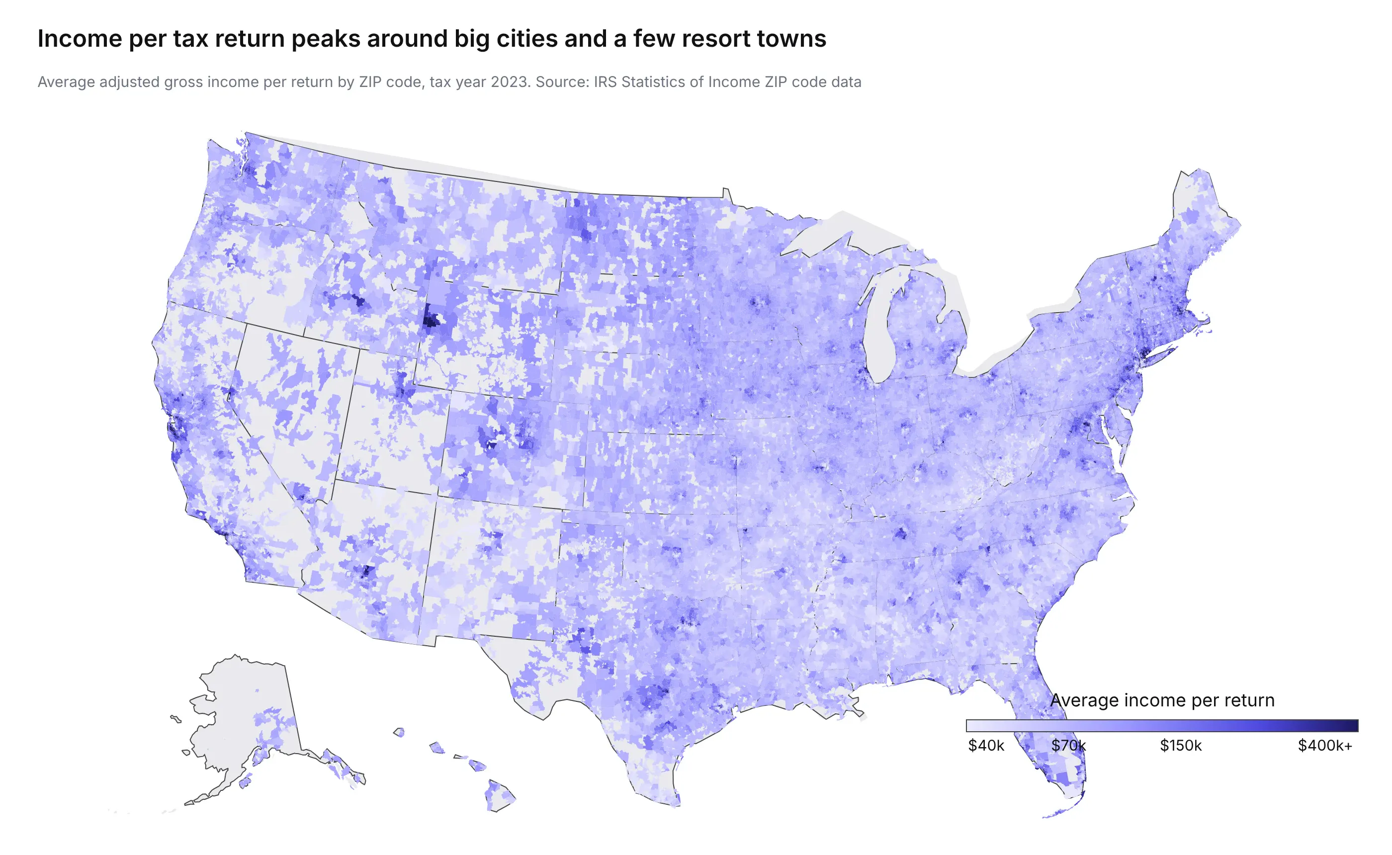
The median ZIP code averages $70,851 per return, and the highest, 33109 (Fisher Island, Florida), averages $3.1 million across 370 returns. A range that wide needs a log color scale, because on a linear one a handful of ZIP codes would take the dark end and everything else would be the same pale color.

2. Residential clean energy credits (energy)

The same IRS file counts returns that claimed the residential clean energy credit, which covers home solar panels, batteries, and similar equipment. Nationally, 1.37 million returns claimed it, 0.89% of all returns.

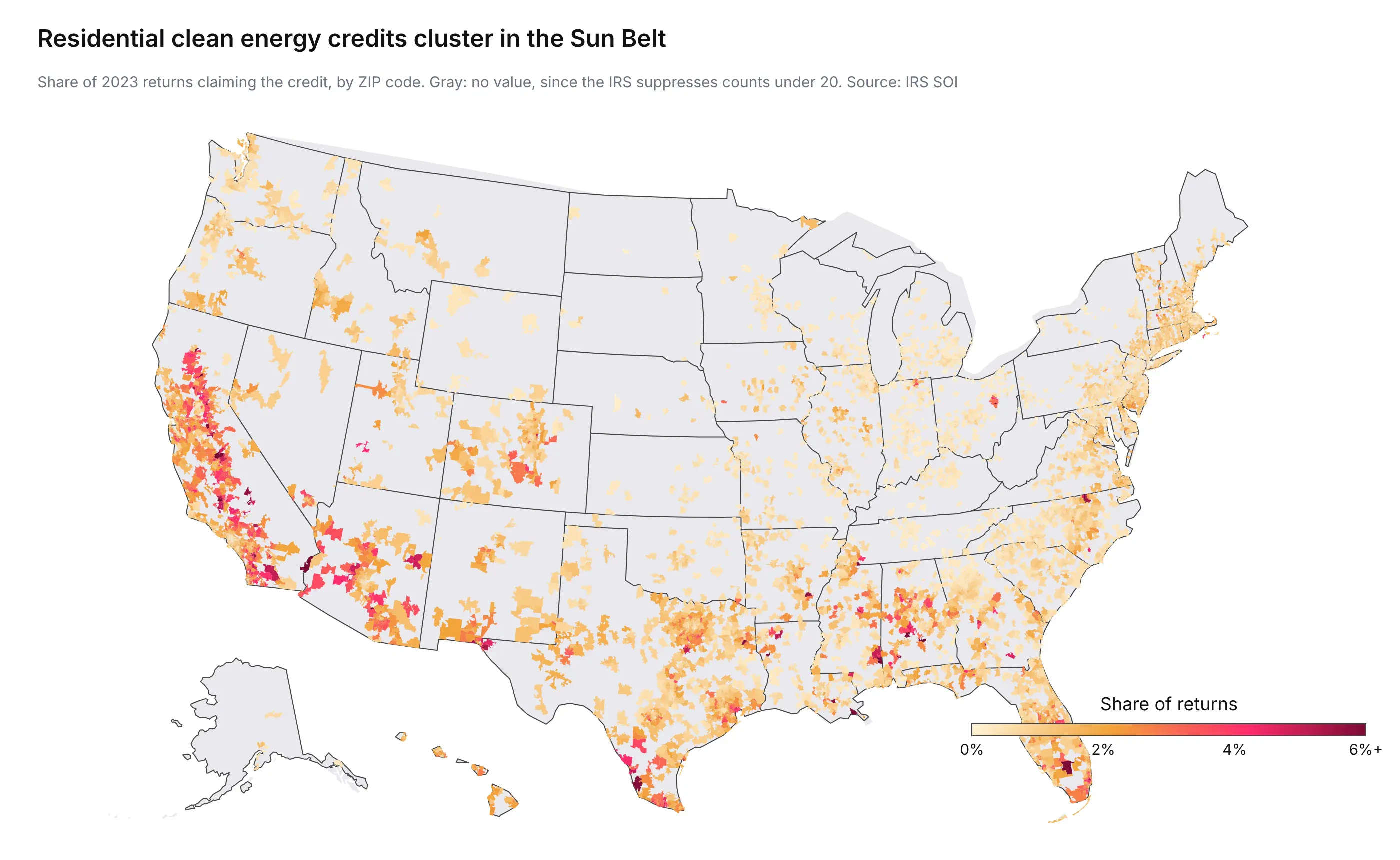
Nevada (2.12% of returns), Hawaii, Florida, Arizona, and California lead by state. The catch is the gray: the IRS suppresses any count under 20 returns, so only 10,222 of 27,689 ZIP codes have a value. A gray ZIP code means "fewer than 20 claims or no data", not zero, and the map has to say so.

3. Residential electricity rates (energy)

OpenEI, the Department of Energy's open data site, publishes the average rates of every utility serving each ZIP code, from the US Energy Information Administration's (EIA) annual utility survey. The typical ZIP code pays 14.2 cents per kilowatt-hour at home.

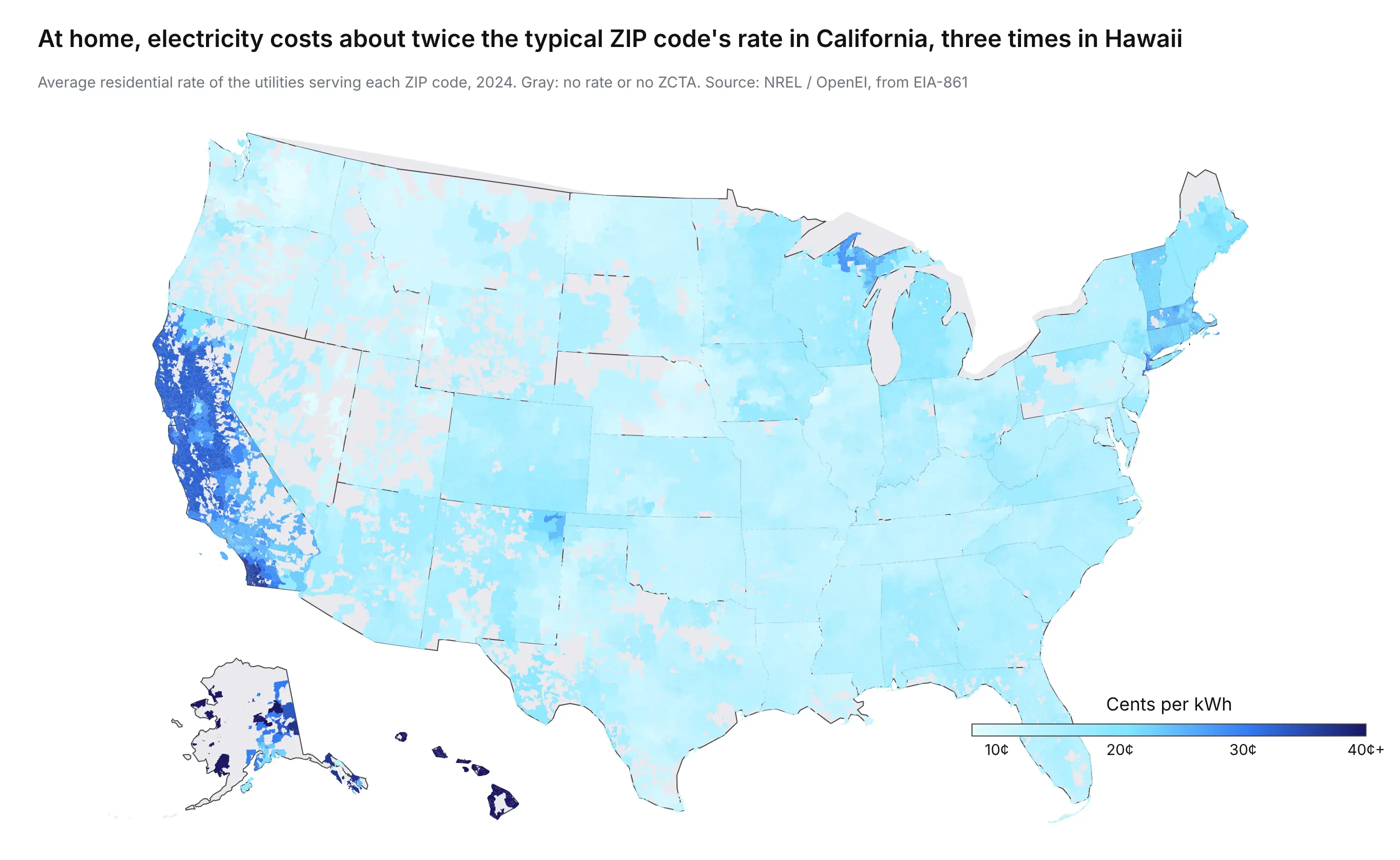
California's ZIP codes have a median of 28.5 cents and Hawaii's 42.9 cents, two and three times the typical rate. The catch: a ZIP code isn't one utility territory. 14,525 of the 38,564 ZIP codes in the file (37.7%) are served by two or more utilities, and one South Carolina ZIP code, 29379, by seven. This map averages them, and a rate shopper or a utility analyst would want each one separately.

4. Recruiting clinical trial sites (pharma)

ClinicalTrials.gov lists every site of every registered trial, with its address. We pulled the 136,509 US sites that are currently recruiting, from 21,767 studies, and counted them by three-digit ZIP code.

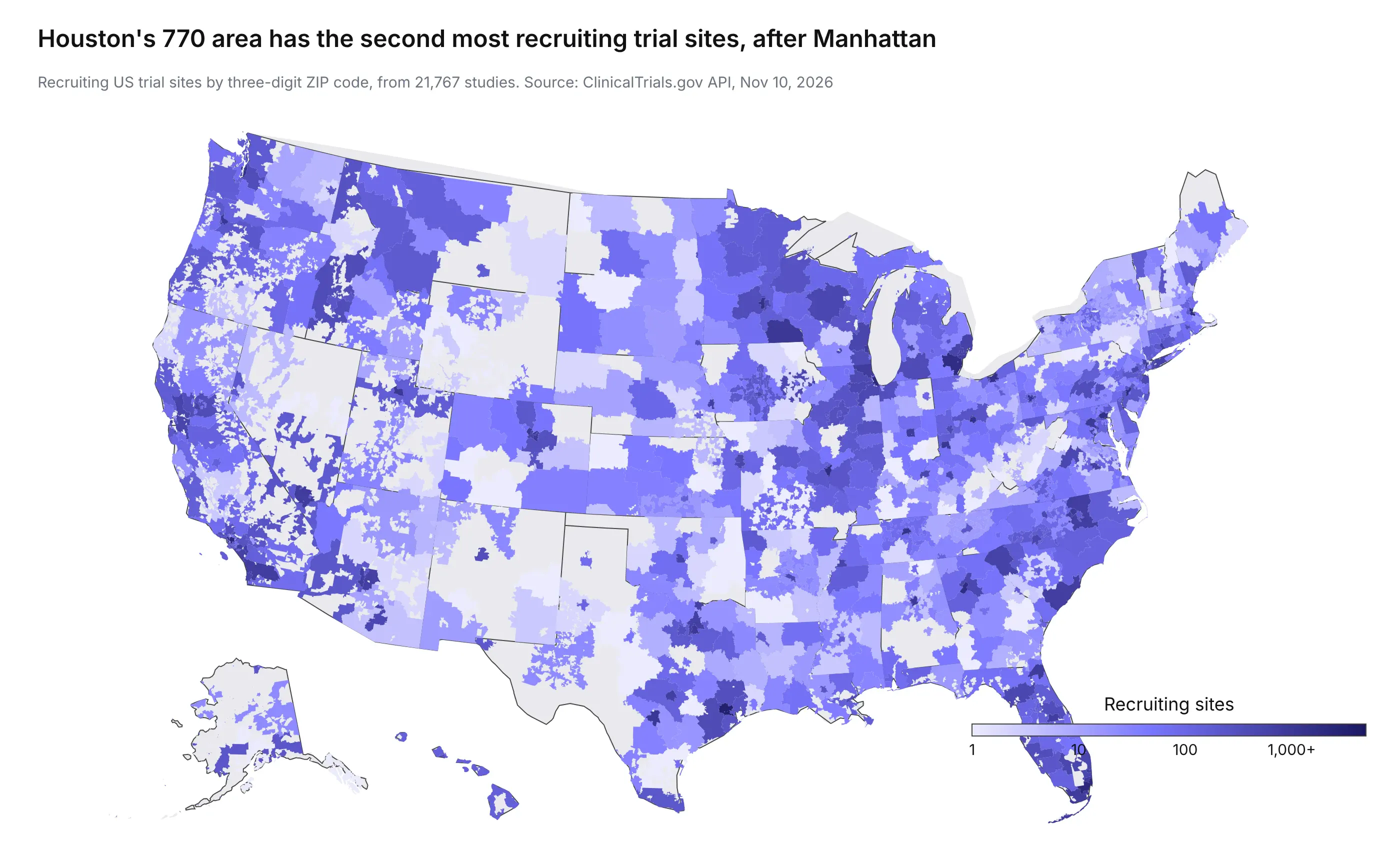
Manhattan's 100 area has the most, 3,671 sites, and Houston's 770 area is second with 3,183, many of them at MD Anderson Cancer Center and Baylor College of Medicine. Three-digit ZIP codes are the right level here for two reasons. Trial sites cluster in a few hospital campuses, so five-digit ZIP codes would show isolated dark specks, and three-digit ZIP codes are also the most detailed ZIP code level that HIPAA's Safe Harbor de-identification rule allows for patient data (more on that below). One cleaning note: the same hospital appears as "MD Anderson Cancer Center" on 356 sites and "M D Anderson Cancer Center" on 234 others, so count by address, not by facility name.

5. Bank branches per tax return (finance)

Counts become comparable once you divide by something. Here, the 77,208 FDIC-insured branches are divided by the number of 2023 tax returns in each three-digit ZIP area, as a stand-in for population.

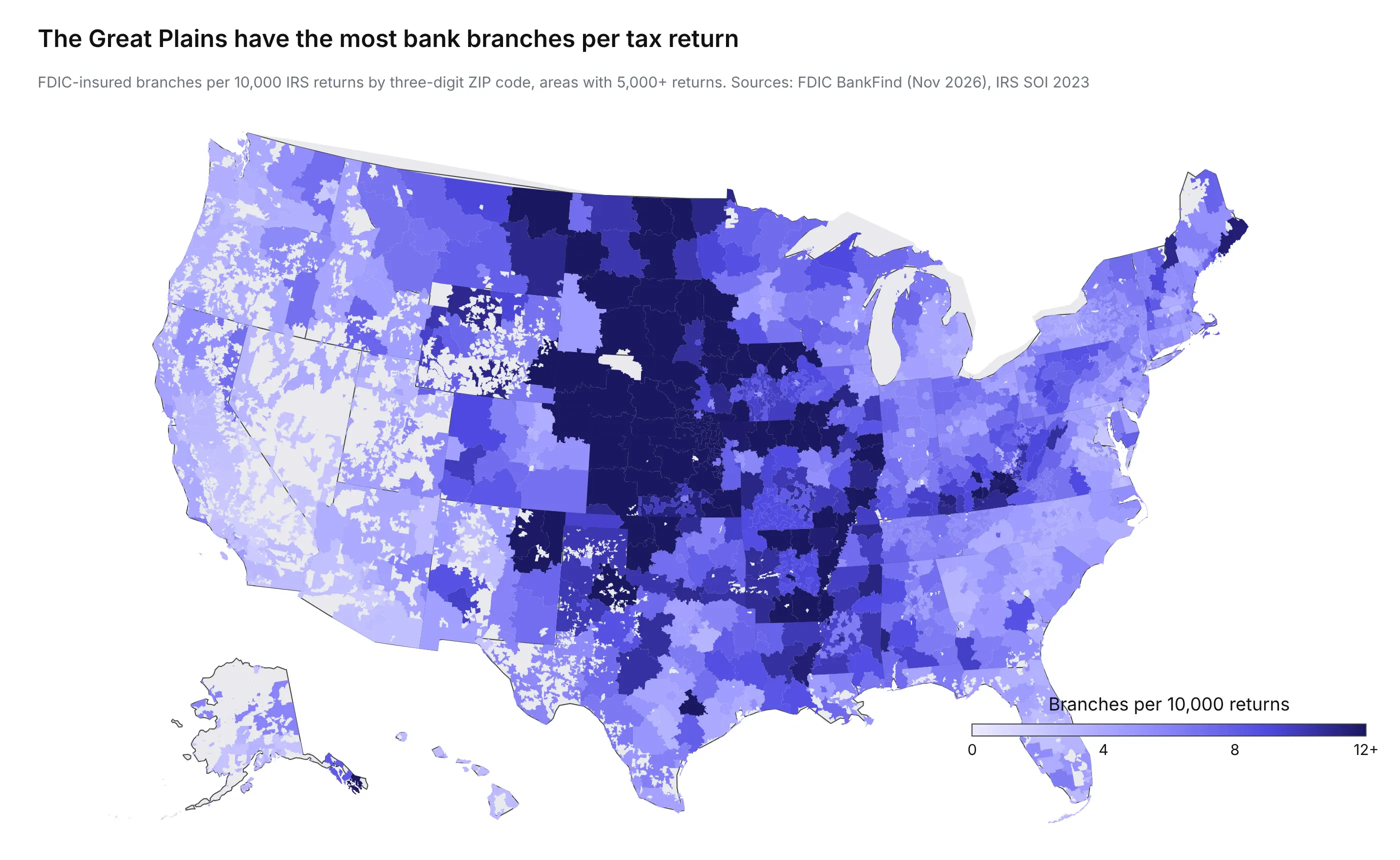
The typical three-digit area has 5.8 branches per 10,000 returns. A north-central Kansas area (669) has 31.5, and the San Bernardino area of California (924) has 1.4. In the Great Plains, many small towns each have a branch serving relatively few people. That pattern is invisible on a map of raw branch counts, which mostly shows where people live.

What makes ZIP code data tricky to graph

ZIP code data looks like any other geographic data, but it breaks several assumptions that people who make maps for a living rely on. These are the ones that matter most, roughly in order of how often they cause a wrong conclusion.

Big ZIP codes get the most ink

Rural ZIP codes are big and urban ones are tiny, so on a filled map the eye goes to the places with the fewest people, and a map colored by raw counts mostly shows where people live. The map below shades every ZCTA by land area, and it looks a lot like a population map for that reason.

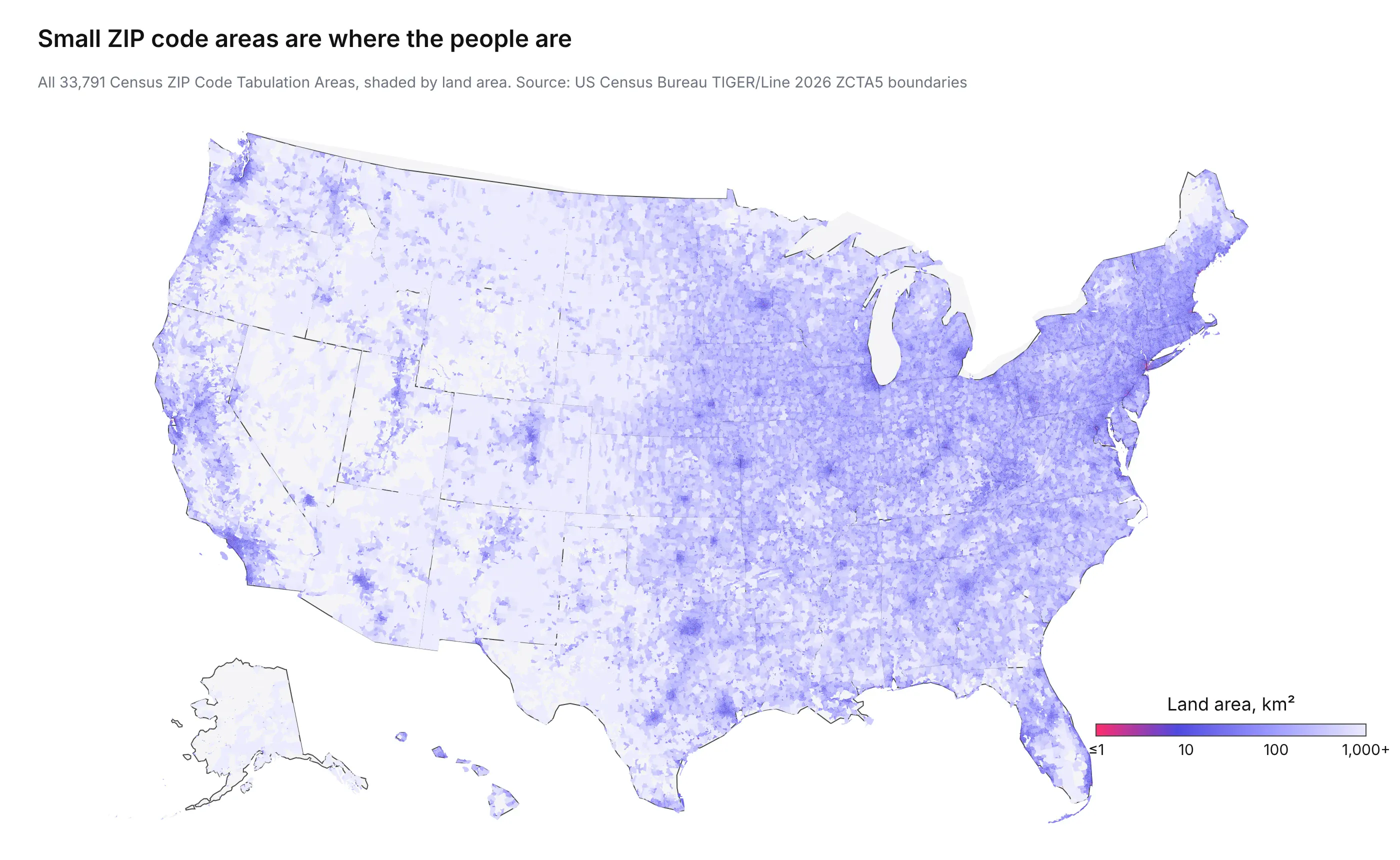
The range is huge. The largest ZCTA, 99557 around Aniak, Alaska, has 35,431 km² of land, more than Maryland. The smallest, 38503 in Cookeville, Tennessee, has 3,551 m², about half a soccer field, and the next three smallest are Manhattan office buildings (10169, 10177, and 10115). The median is 90 km². Divide by population (from the Census tables published by ZCTA) or by your own denominator, such as policies in force, before you compare ZIP codes, as the bank branch example does with tax returns. When the visual weight of big empty ZIP codes still misleads, switch to a bubble map, aggregate to three-digit ZIP codes, or bin into equal-area hexagons.

Some ZIP codes are points, not areas

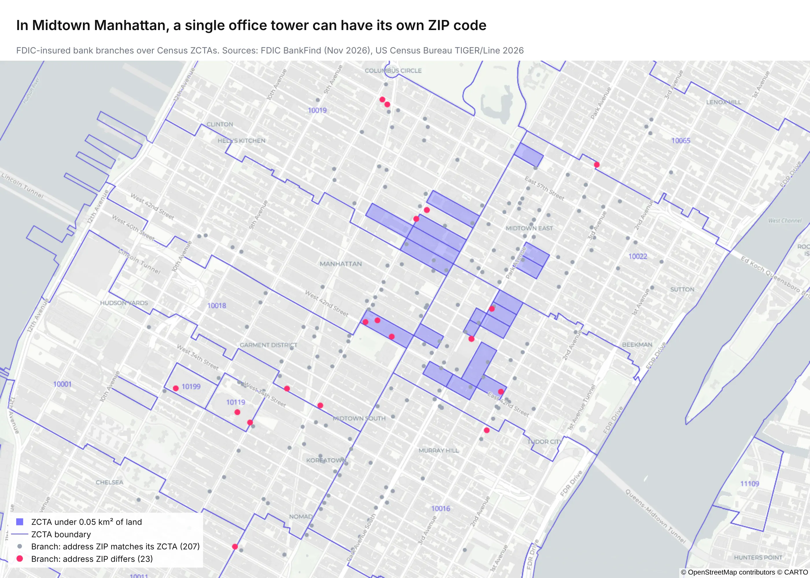
PO box ZIP codes, many single-building and single-company ZIP codes, military ZIP codes, and ZIP codes created after the 2020 Census have no ZCTA, so they drop out of the join. Of the 77,208 FDIC-insured bank branches with coordinates, 147 (0.2%) have a ZIP code with no ZCTA, such as 10041 at 55 Water Street in Manhattan. Always count the rows that didn't join before you trust the map.

Midtown Manhattan shows how strange it gets. Many office towers there have their own ZIP code, and some have a ZCTA no bigger than the building. A branch at 200 Park Avenue has the building's ZIP code, 10166, on its address, but its coordinates fall in the surrounding 10017.

ZIP codes don't nest inside counties and states

Using the Census Bureau's ZCTA-to-county relationship file, we found that 10,180 ZCTAs (30.1%) have land in more than one county, and 117 have more than 1% of their land in a second state. The border between North Dakota and South Dakota has the most of any pair of states, with 16. Towns there are small and far apart, so a rural route often starts at a post office on the other side of the line.

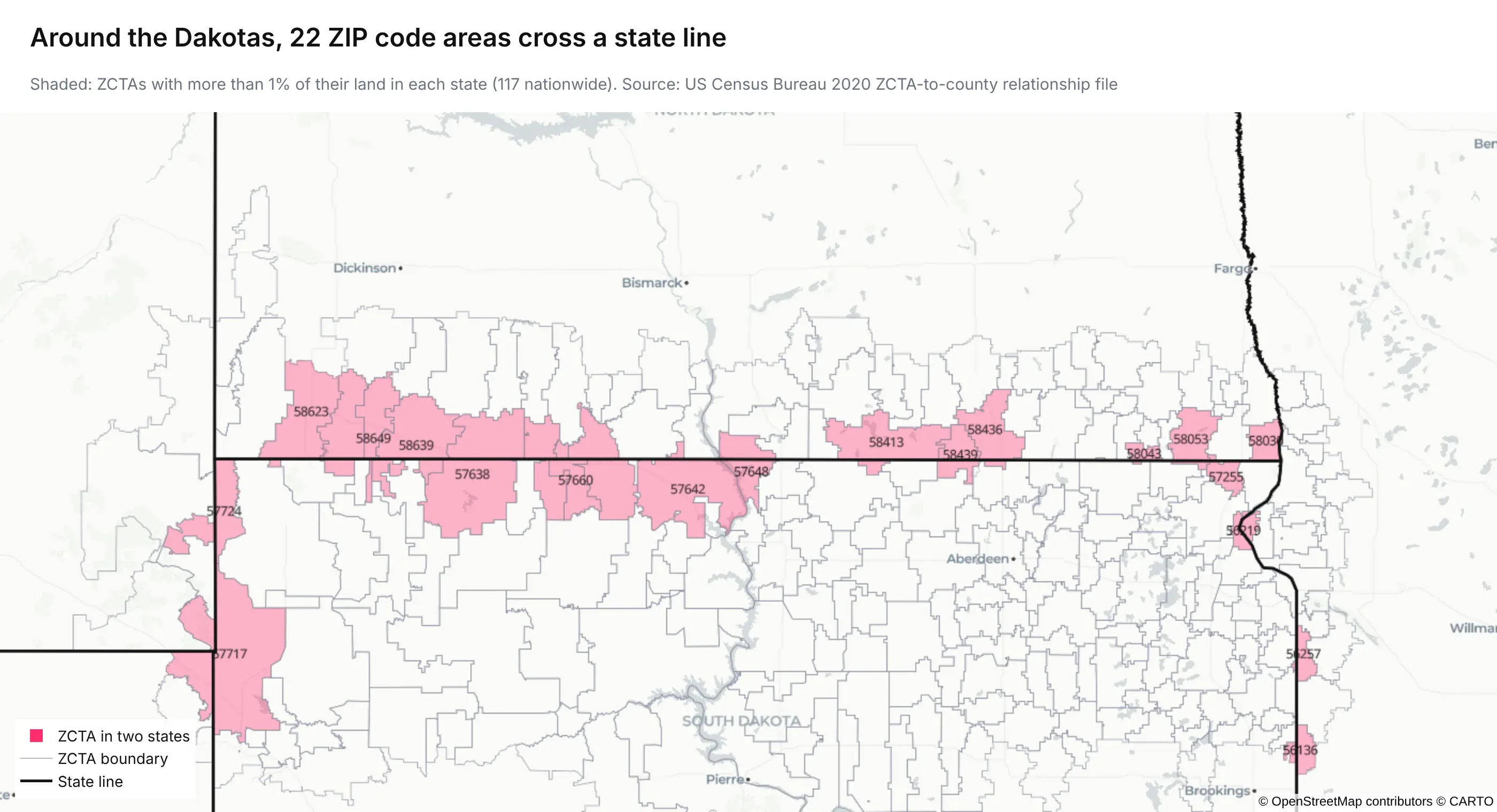
If you roll ZIP code data up to counties or states, for regulatory reporting or a county-level map, split each ZCTA by its share of land (or, better, population) from the relationship file instead of assigning it to one county. For ZIP codes rather than ZCTAs, the Department of Housing and Urban Development (HUD) publishes quarterly USPS ZIP code crosswalk files to counties and census tracts, weighted by address counts.

A fifth of the country is in no ZIP code area

ZCTAs only cover land where people have addresses. Together they hold 7.3 million km² of land, 79.9% of the land in the 50 states, DC, and Puerto Rico, and the rest (national forests, deserts, parts of Alaska) is in no ZCTA at all. On a national map those gaps should look like background, not like a zero, which is why the examples above draw them in a neutral gray rather than the low end of the color scale.

Small numbers are suppressed, and small areas can identify people

Public ZIP code data is often censored on purpose. The IRS drops any count under 20 returns, which is why most ZIP codes are gray on the clean energy credit map. In health data the rule is stricter: under the HIPAA Safe Harbor method for de-identifying patient data, a ZIP code can be kept only as its first three digits, and only if that three-digit area has more than 20,000 people; otherwise it becomes 000 (HHS guidance). If you're mapping patients, claims, or trial participants, plan on three-digit ZIP codes from the start, and expect a few areas to be blank.

One ZIP code can have several values

A ZIP code isn't a unique key for most attributes. In the electricity rate data, 37.7% of ZIP codes are served by more than one utility. The same goes for counties, cities, school districts, and sales territories. Before you color a ZIP code, decide how to combine its values (an average, a customer-weighted average, the largest one) and say which you chose.

The pattern changes with the unit

Aggregating points into areas changes the picture depending on which areas you use, a long-known problem in geography called the modifiable areal unit problem (MAUP). The clinical trial sites show it clearly. At the three-digit level, Houston's 770 area has 3,183 recruiting sites. At the five-digit level, 2,394 of those are in a single ZIP code, 77030, which is the Texas Medical Center, and most of the rest of Houston has few. Neither map is wrong, but they answer different questions, so pick the level that matches the decision the map supports, and check that the main finding holds one level above and below it.

ZIP codes change, and ZCTAs don't

USPS creates, splits, and retires ZIP codes every year, while ZCTAs are redrawn only after each census. Data from 2026 will contain ZIP codes that didn't exist in 2020, and a time series by ZIP code can show a sudden drop that's really a split. For trends, either hold the geography fixed (map everything to 2020 ZCTAs) or use a coarser level that changes less, such as three-digit ZIP codes or counties.

Dos and don'ts for graphing ZIP codes

A short checklist of everything above.

Do:

• Read ZIP codes as text and pad them to five digits with leading zeros.
• Count and list the rows that didn't join to a shape before you draw anything.
• Divide by a denominator (population, households, returns, or accounts) when you compare ZIP codes.
• Use a log or quantile color scale for skewed values like income or counts.
• Draw areas with no data or no ZCTA in a neutral gray, and say what gray means.
• Use three-digit ZIP codes for patient data, for national maps, and for trends over time.
• Split ZIP codes across counties with a crosswalk when you roll up.
• Put the data source, the year, and the geography (ZCTA or ZIP code) in the subtitle.

Don't:

• Treat ZIP codes as numbers, on an axis or anywhere else.
• Assume every ZIP code has a shape, or that every shape has one ZIP code's worth of data.
• Assign a ZIP code to a single county or state without checking.
• Compare raw counts across ZIP codes of very different sizes.
• Read meaning into big rural ZIP codes just because they cover a lot of the map.
• Show five-digit ZIP codes for health data with small counts.

Are free ZIP code shapes accurate enough?

For a heat map or a bubble map, yes. We checked them two ways.

Against real addresses. We placed all 77,208 FDIC-insured bank branches with coordinates into the ZCTAs, and 96.8% (74,701) landed in the ZCTA with the same code as the ZIP code on their address. Of the rest, 147 have no ZCTA and 2,360 fall in a neighboring one, either near an edge, in a building with its own ZIP code, or at coordinates the source geocoded to the wrong place.

Against the USPS boundaries. We didn't buy the USPS product, but USPS publishes a free sample of 10 ZIP codes in western Puerto Rico, and we compared it with the matching ZCTAs.

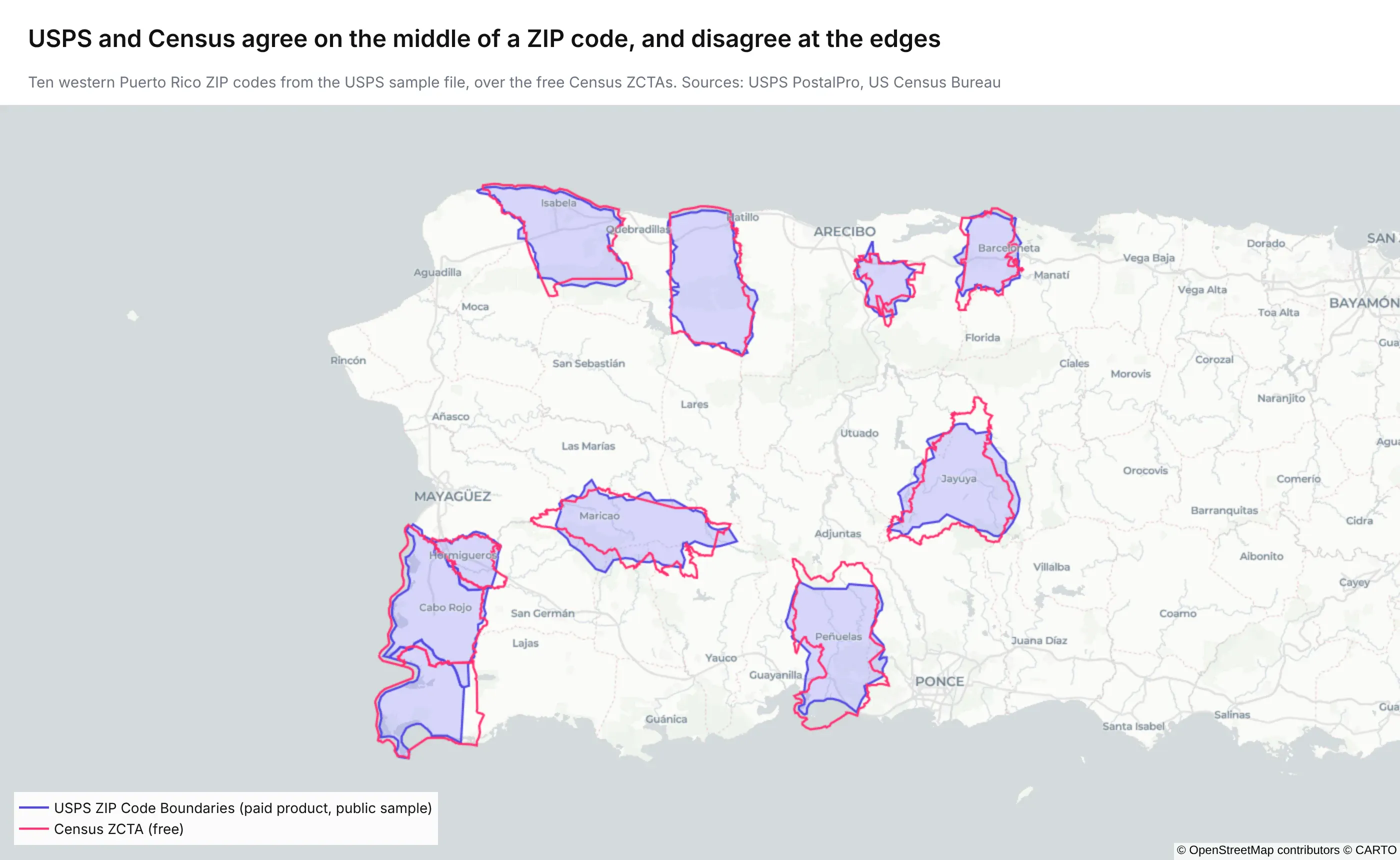
Of the 783 km² that both sources cover, 98.5% is assigned the same ZIP code by both. The shapes themselves differ more at the edges: the intersection over union (IoU), the overlapping area divided by the combined area of the two shapes, ranges from 0.65 for Boquerón to 0.88 for Camuy, with a median of 0.74. That's mostly because the two handle coastlines, forests, and empty land differently, so the ZCTAs cover 932 km² in total and the USPS polygons 865 km².

So a graph built on ZCTAs will put nearly every record in the right ZIP code. If you're computing a ZIP code's area, counting what falls near its edge, or working with ZIP codes created since 2020, the paid USPS boundaries are worth a look.

How to graph ZIP codes with Plotly Studio or a coding agent

If you'd rather describe the graphs than write them, give Plotly Studio or a coding agent such as Claude Code your data and a prompt like this one:

Download the Census 2026 ZCTA shapefile from https://www2.census.gov/geo/tiger/TIGER2026/ZCTA520/tl_2026_us_zcta520.zip. Join it to `claims.csv` on the `zip` column (read it as text and pad ZIP codes to five digits). Build a Dash app with a Plotly tile choropleth map of claims per 1,000 residents by ZCTA, a bar chart of the top 20 ZIP codes, a dropdown to pick a state, and a table of ZIP codes in the CSV that have no ZCTA so we can see what didn't match. Simplify the polygons so the map stays fast.

Asking for the list of unmatched ZIP codes is the important part, because it tells you how much of your data the map leaves out before anyone draws conclusions from it.

Summary

Graphing ZIP codes in Python takes your data, the free Census ZCTA shapefile for maps, and one Plotly call: px.choropleth_map for a heat map, px.scatter_map for a bubble map, or px.bar with a category axis for a chart. The free shapes are close enough for nearly every map: they matched 96.8% of bank branch addresses, and they agreed with the USPS sample on 98.5% of shared land. Most of the work is in the details: keep ZIP codes as text, check which ones didn't join, map rates instead of counts, gray out what's missing or suppressed, use three-digit ZIP codes for patient data and trends, and split ZIP codes that cross county lines when you roll up. The new USPS boundaries are there for when you need quarterly updates or exact edges.