

Display Line Animation
Create the initial animated line object. Then, use a loop to add 1,000 points to the line. After adding each new point, use drawnow to display the new point on the screen.
h = animatedline;
axis([0,4*pi,-1,1])

x = linspace(0,4*pi,1000);
y = sin(x);
for k = 1:length(x)
    addpoints(h,x(k),y(k));
    drawnow
end


fig2plotly()


For faster rendering, add more than one point to the line each time through the loop or use drawnow limitrate.
Query the points of the line.
[xdata,ydata] = getpoints(h);


fig2plotly()
Clear the points from the line.
clearpoints(h)
drawnow


fig2plotly()


Specify Animated Line Color
Set the color of the animated line to red and set its line width to 3 points.
x = [1 2];
y = [1 2];
h = animatedline(x,y,'Color','r','LineWidth',3);

fig2plotly()

Set Maximum Number of Points
Limit the number of points in the animated line to 100. Use a loop to add one point to the line at a time. When the line contains 100 points, adding a new point to the line deletes the oldest point.
h = animatedline('MaximumNumPoints',100);
axis([0,4*pi,-1,1])

x = linspace(0,4*pi,1000);
y = sin(x);
for k = 1:length(x)
    addpoints(h,x(k),y(k));
    drawnow
end


fig2plotly()


Add Points in Sets for Fast Animation
Use a loop to add 100,000 points to an animated line. Since the number of points is large, adding one point to the line each time through the loop might be slow. Instead, add 100 points to the line each time through the loop for a faster animation.
h = animatedline;
axis([0,4*pi,-1,1])

numpoints = 100000;
x = linspace(0,4*pi,numpoints);
y = sin(x);
for k = 1:100:numpoints-99
    xvec = x(k:k+99);
    yvec = y(k:k+99);
    addpoints(h,xvec,yvec)
    drawnow
end


fig2plotly()


Another technique for creating faster animations is to use drawnow limitrate instead of drawnow.
Use drawnow limitrate for Fast Animation
Use a loop to add 100,000 points to an animated line. Since the number of points is large, using drawnow to display the changes might be slow. Instead, use drawnow limitrate for a faster animation.
h = animatedline;
axis([0,4*pi,-1,1])

numpoints = 100000;
x = linspace(0,4*pi,numpoints);
y = sin(x);
for k = 1:numpoints
    addpoints(h,x(k),y(k))
    drawnow limitrate
end


fig2plotly()

Control Animation Speed
Control the animation speed by running through several iterations of the animation loop before drawing the updates on the screen. Use this technique when drawnow is too slow and drawnow limitrate is too fast.
For example, update the screen every 1/30 seconds. Use the tic and toc commands to keep track of how much time passes between screen updates.
h = animatedline;
axis([0,4*pi,-1,1])
numpoints = 10000;
x = linspace(0,4*pi,numpoints);
y = sin(x);
a = tic; % start timer
for k = 1:numpoints
    addpoints(h,x(k),y(k))
    b = toc(a); % check timer
    if b > (1/30)
        drawnow % update screen every 1/30 seconds
        a = tic; % reset timer after updating
    end
end
drawnow % draw final frame


fig2plotly()


A smaller interval updates the screen more often and results in a slower animation. For example, use b > (1/1000) to slow down the animation.
Create Comet Plot
Create a comet plot of data in y versus data in x. Create y as a vector of sine function values for input values between 0 and 2π. Create x as a vector of cosine function values for input values between 0 and 2π. Use an increment of π/100 between the values. Then, plot the data.
t = 0:pi/100:2*pi;
y = sin(t);
x = cos(t);
comet(x,y)

fig2plotly()

Control Comet Body Length
Create a comet plot and specify the comet body length by setting the scale factor input p. The comet body is a trailing segment in a different color that follows the head before fading.
Create x and y as vectors of trigonometric functions with input values from 0 to 4π. Specify p as 0.5 so that the comet body length is 0.5*length(y). Then, plot the data.
t = 0:pi/50:4*pi;
x = -sin(t) - sin(t/2);
y = -cos(t) + cos(t/2);
p = 0.5;
comet(x,y,p)

fig2plotly()

Create Plots in Specified Axes
Create two comet plots in a tiled chart layout by specifying the target axes for each plot. Create two data sets, x1 and y1 and x2 and y2 as vectors of trigonometric functions with input values from 0 to 4π. Specify the body length scale factor p as 0.25 so that the body length is 0.25*length(y).
t = 0:pi/20:4*pi;
x1 = -cos(t) + cos(t/2);
y1 = -sin(t) - sin(t/2);
x2 =  cos(t) - cos(t/2);
y2 = -sin(t) - sin(t/2);
p = 0.25;
Store the two Axes objects as ax1 and ax2. Specify the target axes for each comet plot by including the Axes object as the first input argument to comet.
tiledlayout(1,2);
ax1 = nexttile;
ax2 = nexttile;

comet(ax1,x1,y1,p)
comet(ax2,x2,y2,p)

fig2plotly()

Create 3-D Comet Plot
Create a comet plot of the data in z versus the data in x and y. Use the peaks function to load x, y, and z data in matrix forms. Convert the data into vector arrays. Then, plot the data.
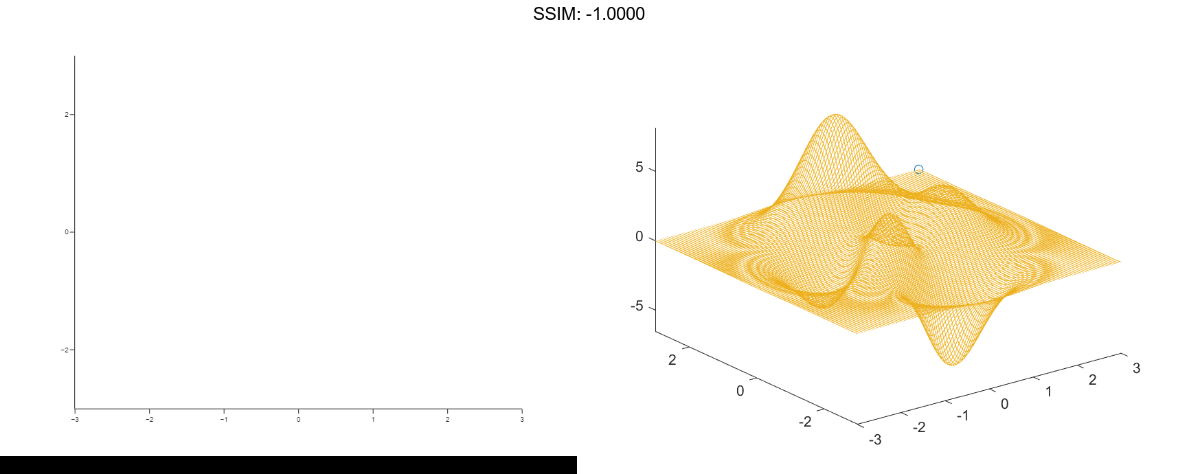
[xmat,ymat,zmat] = peaks(100);
xvec = xmat(:);
yvec = ymat(:);
zvec = zmat(:);
comet3(xvec,yvec,zvec)

fig2plotly()

Control Comet Body Length
Create a comet plot and specify the comet body length by setting the scale factor input p. The comet body is a trailing segment in a different color that follows the head before fading.
Use the peaks function to load x, y, and z data in matrix forms. Convert the data into vector arrays. Specify p as 0.5 so that the body length is 0.5*length(y). Then, plot the data.
[xmat,ymat,zmat] = peaks(100);
xvec = xmat(:);
yvec = ymat(:);
zvec = zmat(:);
p = 0.5;
comet3(xvec,yvec,zvec,p)

fig2plotly()
Plot Data in Specified Axes
Create two comet plots in a tiled chart layout by specifying the target axes for each plot.
Use the peaks function to load x, y, and z data in matrix forms. Convert the data into vector arrays. Specify the body length scale factor p as 0.25 so that the body length is 0.5*length(y).
[xmat,ymat,zmat] = peaks(50);
xvec = xmat(:);
yvec = ymat(:);
zvec = zmat(:);
p = 0.25;
Store the two Axes objects as ax1 and ax2. Specify the target axes for each comet plot by including the Axes object as the first input argument to comet.
tiledlayout(1,2);
ax1 = nexttile;
ax2 = nexttile;

comet3(ax1,xvec,yvec,zvec,p)
comet3(ax2,yvec,xvec,zvec,p)

fig2plotly()

Animate Flow Without Displaying Streamlines
This example uses streamlines in the z = 5 plane to animate the flow along these lines with stream particles.
load wind
figure
daspect([1,1,1]);
view(2)
[verts,averts] = streamslice(x,y,z,u,v,w,[],[],5);
sl = streamline([verts averts]);
axis tight manual off;
set(sl,'Visible','off')
iverts = interpstreamspeed(x,y,z,u,v,w,verts,.05);
zlim([4.9,5.1]);
streamparticles(iverts, 200, ...
    'Animate',15,'FrameRate',40, ...
    'MarkerSize',10,'MarkerFaceColor',[0 .5 0])

fig2plotly()
plot00animateflowwithoutdisplaying_streamlines