

MATLAB fsurf in MATLAB®
Learn how to make 8 fsurf charts in MATLAB, then publish them to the Web with Plotly.
3-D Surface Plot of Expression
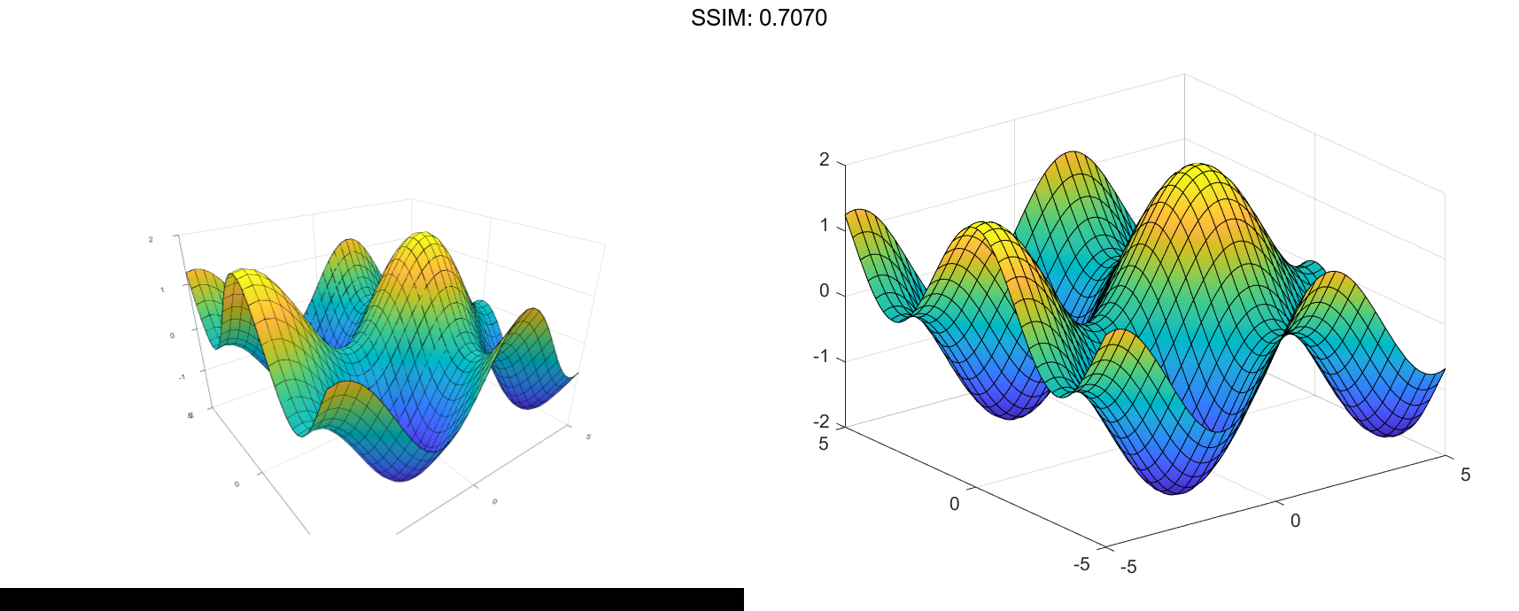
Plot the expression sin(x)+cos(y) over the default interval -5<x<5 and -5<y<5.
fsurf(@(x,y) sin(x)+cos(y))

fig2plotly()

Specify Interval of Surface Plot and Plot Piecewise Expression
Plot the piecewise expression
erf(x)+cos(y) -5<x<0
sin(x)+cos(y) 0<x<5
over -5<y<5.
Specify the plotting interval as the second input argument of fsurf. When you plot multiple surfaces over different intervals in the same axes, the axis limits adjust to include all the data.
f1 = @(x,y) erf(x)+cos(y);
fsurf(f1,[-5 0 -5 5])
hold on
f2 = @(x,y) sin(x)+cos(y);
fsurf(f2,[0 5 -5 5])
hold off

fig2plotly()


Parameterized Surface Plot
Plot the parameterized surface
x=rcos(u)sin(v)
y=rsin(u)sin(v)
z=rcos(v)
where r=2+sin(7u+5v)
for 0<u<2π and 0<v<π. Add light to the surface using camlight.
r = @(u,v) 2 + sin(7.*u + 5.*v);
funx = @(u,v) r(u,v).*cos(u).*sin(v);
funy = @(u,v) r(u,v).*sin(u).*sin(v);
funz = @(u,v) r(u,v).*cos(v);
fsurf(funx,funy,funz,[0 2*pi 0 pi])
camlight

fig2plotly()


Add Title and Axis Labels and Format Ticks
For x and y from -2π to 2π, plot the 3-D surface ysin(x)-xcos(y). Add a title and axis labels and display the axes outline.
fsurf(@(x,y) y.*sin(x)-x.*cos(y),[-2*pi 2*pi])
title('ysin(x) - xcos(y) for x and y in [-2\pi,2\pi]')
xlabel('x');
ylabel('y');
zlabel('z');
box on

fig2plotly()


Set the x-axis tick values and associated labels using the XTickLabel and XTick properties of axes object. Access the axes object using gca. Similarly, set the y-axis tick values and associated labels.
ax = gca;
ax.XTick = -2*pi:pi/2:2*pi;
ax.XTickLabel = {'-2\pi','-3\pi/2','-\pi','-\pi/2','0','\pi/2','\pi','3\pi/2','2\pi'};

ax.YTick = -2*pi:pi/2:2*pi;
ax.YTickLabel = {'-2\pi','-3\pi/2','-\pi','-\pi/2','0','\pi/2','\pi','3\pi/2','2\pi'};

fig2plotly()


Specify Surface Properties
Plot the parametric surface x=usin(v), y=-ucos(v), z=v with different line styles for different values of v. For -5<v<-2, use a dashed green line for the surface edges. For -2<v<2, turn off the edges by setting the EdgeColor property to 'none'.
funx = @(u,v) u.*sin(v);
funy = @(u,v) -u.*cos(v);
funz = @(u,v) v;

fsurf(funx,funy,funz,[-5 5 -5 -2],'--','EdgeColor','g')
hold on
fsurf(funx,funy,funz,[-5 5 -2 2],'EdgeColor','none')
hold off

fig2plotly()


Modify Surface After Creation
Plot the parametric surface
x=e-|u|/10sin(5|v|)
y=e-|u|/10cos(5|v|)
z=u.
Assign the parameterized function surface object to a variable.
x = @(u,v) exp(-abs(u)/10).sin(5abs(v)); y = @(u,v) exp(-abs(u)/10).cos(5abs(v)); z = @(u,v) u; fs = fsurf(x,y,z)


fs =
  ParameterizedFunctionSurface with properties:

    XFunction: @(u,v)exp(-abs(u)/10).*sin(5*abs(v))
    YFunction: @(u,v)exp(-abs(u)/10).*cos(5*abs(v))
    ZFunction: @(u,v)u
    EdgeColor: [0 0 0]
    LineStyle: '-'
    FaceColor: 'interp'

  Show all properties
fs.URange = [-30 30];

fig2plotly()


fs.FaceAlpha = .5;

fig2plotly()
Show Contours Below Surface Plot
Show contours below a surface plot by setting the 'ShowContours' option to 'on'.
f = @(x,y) 3*(1-x).^2.*exp(-(x.^2)-(y+1).^2)...
    - 10*(x/5 - x.^3 - y.^5).*exp(-x.^2-y.^2)...
    - 1/3*exp(-(x+1).^2 - y.^2);
fsurf(f,[-3 3],'ShowContours','on')

fig2plotly()


Control Resolution of Surface Plot
Control the resolution of a surface plot using the 'MeshDensity' option. Increasing 'MeshDensity' can make smoother, more accurate plots while decreasing it can increase plotting speed.
Create two plots in a tiled chart layout. In the first plot, display the parametric surface x=sin(s), y=cos(s), z=(t/10)sin(1/s). The surface has a large gap. Fix this issue by increasing the 'MeshDensity' to 40 in the second plot. fsurf fills the gap, showing that by increasing 'MeshDensity' you increased the resolution.
tiledlayout(2,1)
nexttile
fsurf(@(s,t) sin(s), @(s,t) cos(s), @(s,t) t/10.*sin(1./s))
view(-172,25)
title('Default MeshDensity = 35')

nexttile
fsurf(@(s,t) sin(s), @(s,t) cos(s), @(s,t) t/10.*sin(1./s),'MeshDensity',40)
view(-172,25)
title('Increased MeshDensity = 40')

fig2plotly()

