MATLAB stem3 in MATLAB®
Learn how to make 11 stem3 charts in MATLAB, then publish them to the Web with Plotly.
Row Vector Input
Create a 3-D stem plot of cosine values between -π/2 and π/2 with a row vector input.
figure
X = linspace(-pi/2,pi/2,40);
Z = cos(X);
stem3(Z)

fig2plotly()
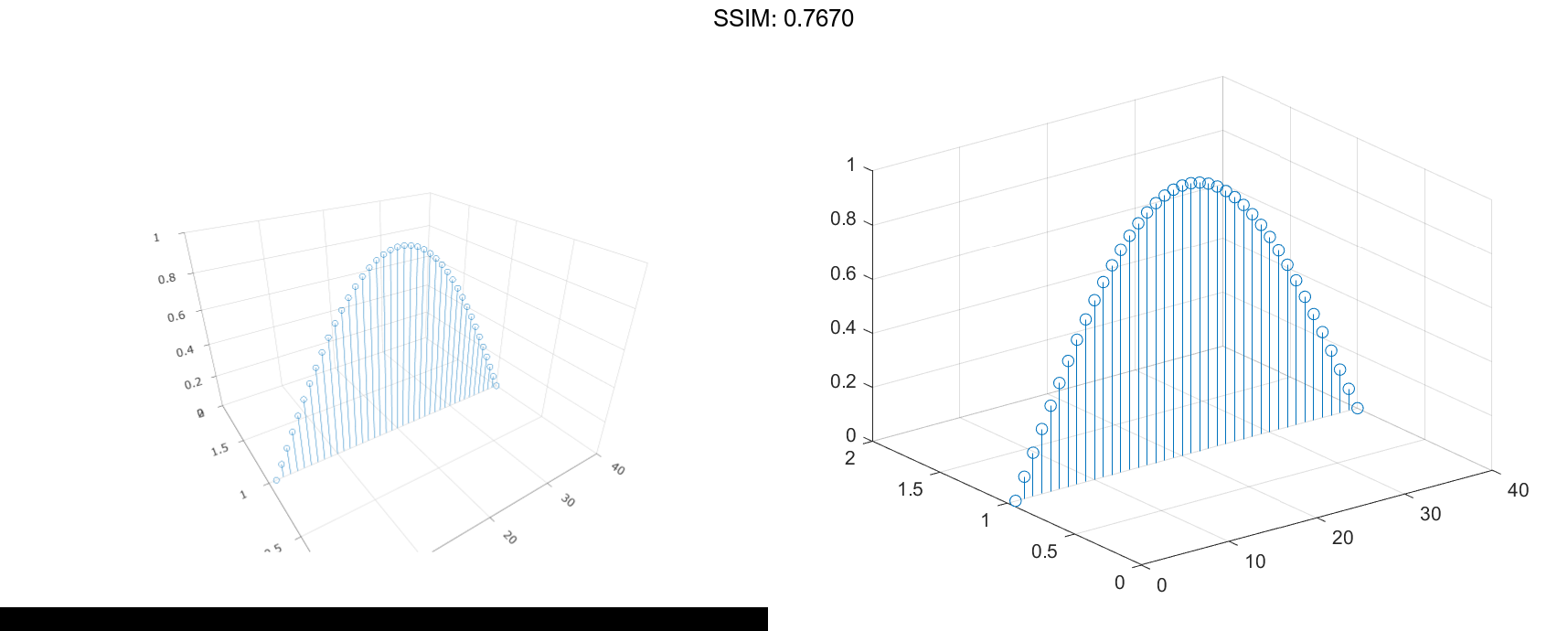
stem3 plots elements of Z against the same y value at equally space x values.
Column Vector Input
Create a 3-D stem plot of cosine values between -π/2 and π/2 with a column vector input.
figure
X = linspace(-pi/2,pi/2,40)';
Z = cos(X);
stem3(Z)

fig2plotly()
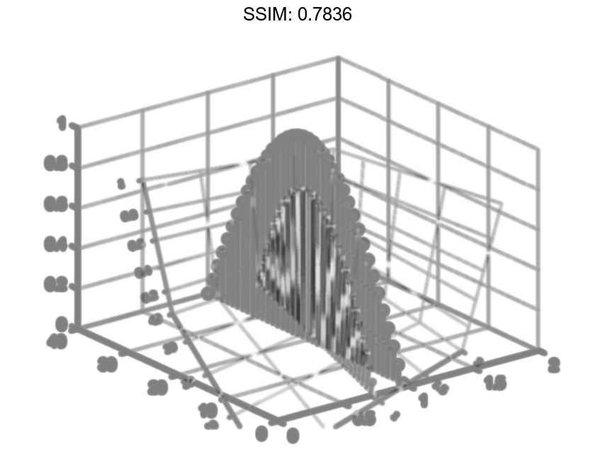
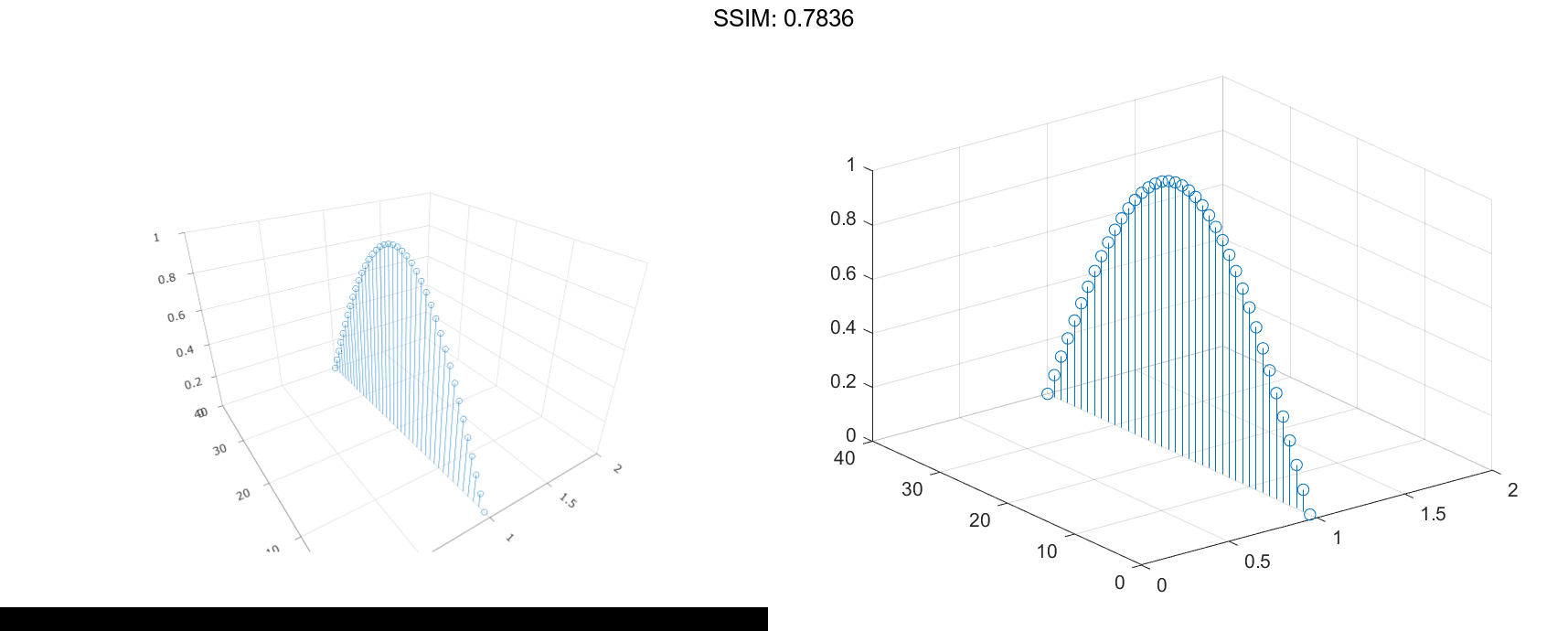
stem3 plots elements of Z against the same x value at equally space y values.
Matrix Input
Create a 3-D stem plot of sine and cosine values between -π/2 and π/2 with a matrix input.
figure
X = linspace(-pi/2,pi/2,40);
Z = [sin(X); cos(X)];
stem3(Z)

fig2plotly()
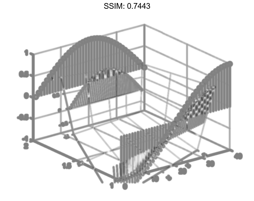
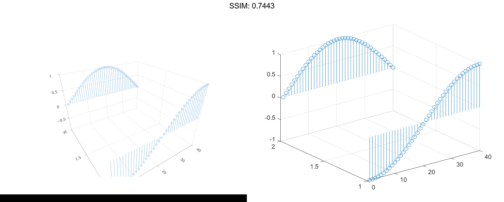
stem3 plots each row of Z against the same y value at equally space x values.
Specify Stem Locations with Vector Inputs
Create a 3-D stem plot and specify the stem locations along a curve. Use view to adjust the angle of the axes in the figure.
figure
X = linspace(-5,5,60);
Y = cos(X);
Z = X.^2;
stem3(X,Y,Z)
view(-8,30)

fig2plotly()
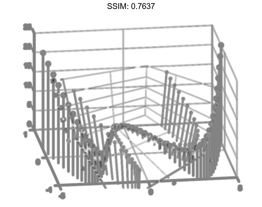
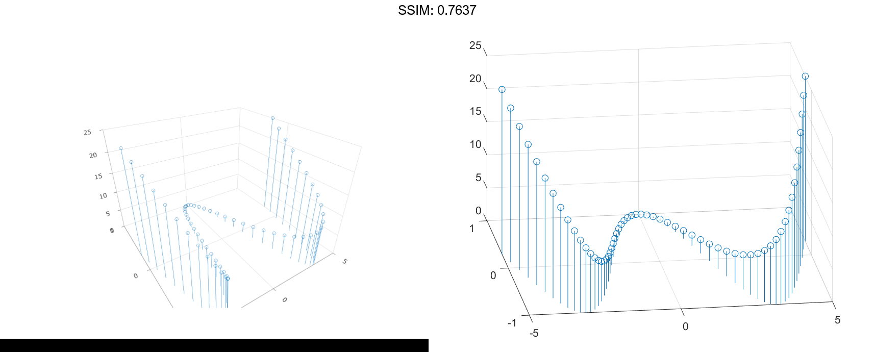
X and Y determine the stem locations. Z determines the marker heights.
Specify Stem Locations with Matrix Inputs
Create a 3-D stem plot with matrix data and specify the stem locations in the xy-plane.
figure
[X,Y] = meshgrid(0:.1:1);
Z = exp(X+Y);
stem3(X,Y,Z)

fig2plotly()
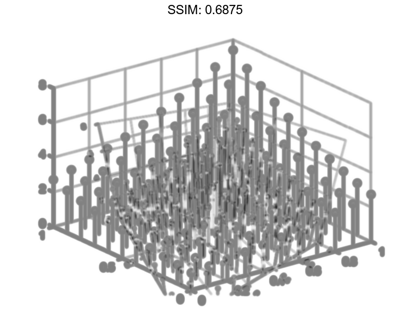
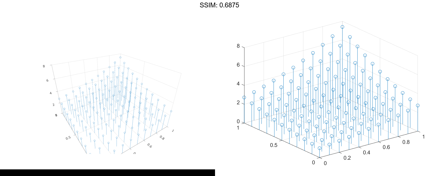
X and Y determine the stem locations. Z determines the marker heights.
Fill in Markers
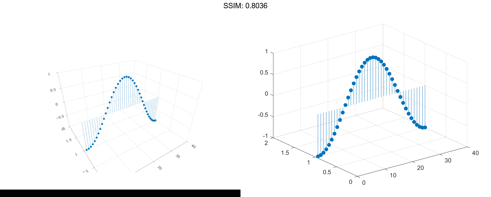
Create a 3-D stem plot of cosine values between -π and π and fill in the markers.
X = linspace(-pi,pi,40);
Z = cos(X);
stem3(Z,'filled')

fig2plotly()
Line Style, Marker Symbol, and Color Options
Create a 3-D stem plot of cosine values between -π and π. Use a dashed line style for the stem, set the marker symbols to stars, and set the color to magenta.
figure
X = linspace(-pi,pi,40);
Z = cos(X);
stem3(Z,'--*m')

fig2plotly()
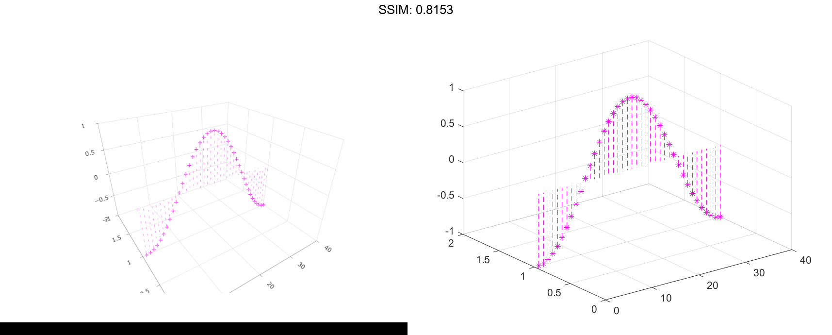
To specify only two of the three LineSpec options, omit the third option from the character vector. For example, '*m' sets the marker symbol and the color and uses the default line style.
Line Style, Marker Symbol, and Color Options
Create a 3-D stem plot and specify the stem locations along a circle. Set the stem to a dotted line style, the marker symbols to stars, and the color to magenta.
figure
theta = linspace(0,2*pi);
X = cos(theta);
Y = sin(theta);
Z = theta;
stem3(X,Y,Z,':*m')

fig2plotly()
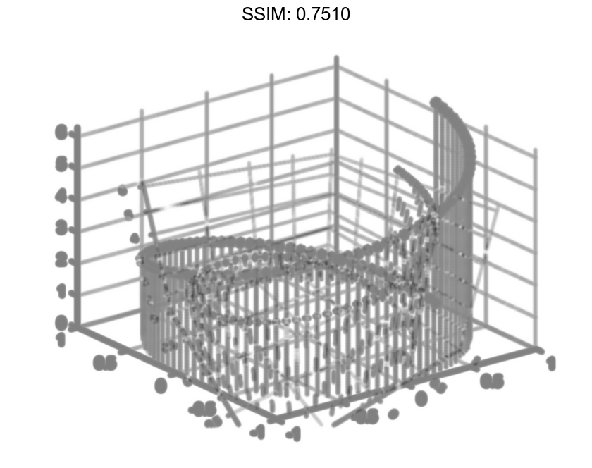
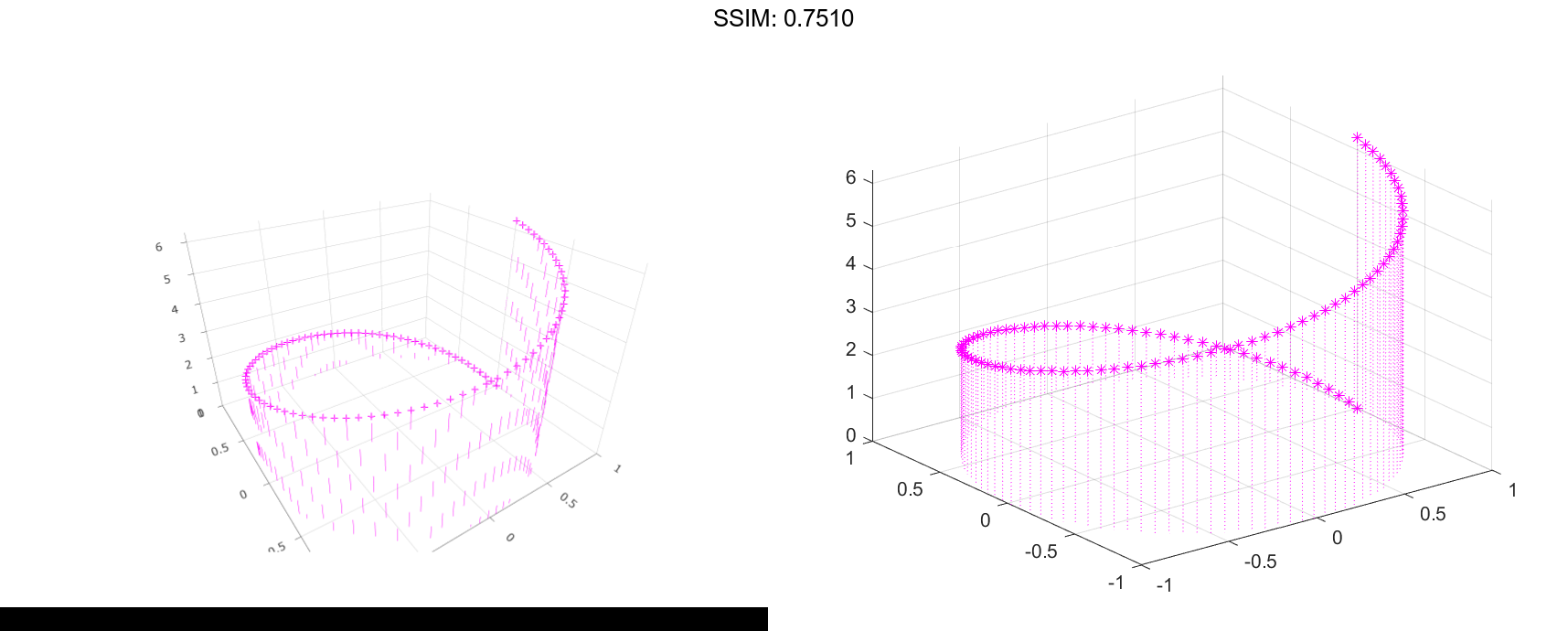
X and Y determine the stem locations. Z determines the marker heights.
Additional Style Options
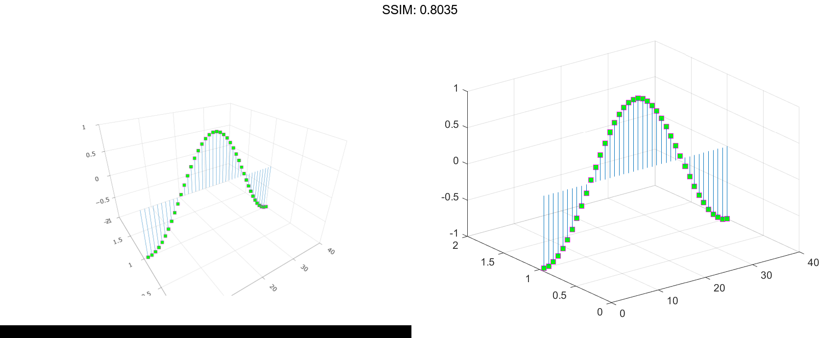
Create a 3-D stem plot of cosine values between -π and π. Set the marker symbols to squares with green faces and magenta edges.
figure
X = linspace(-pi,pi,40);
Z = cos(X);
stem3(Z,'Marker','s',...
     'MarkerEdgeColor','m',...
     'MarkerFaceColor','g')

fig2plotly()

Stem Plot in Specific Axes
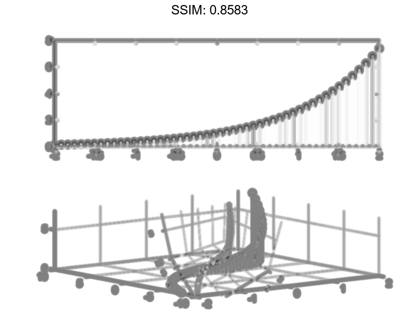
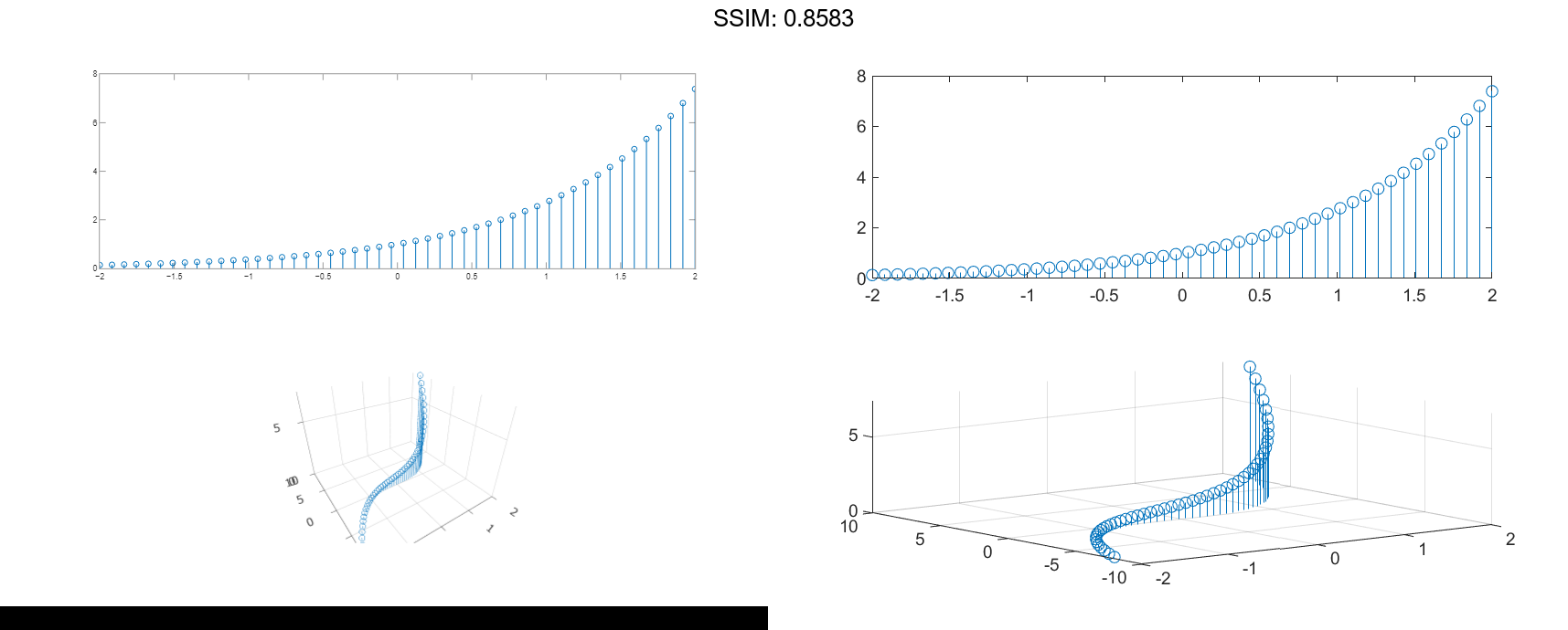
Starting in R2019b, you can display a tiling of plots using the tiledlayout and nexttile functions. Call the tiledlayout function to create a 2-by-1 tiled chart layout. Call the nexttile function to create the axes objects ax1 and ax2. Create separate stem plots in the axes by specifying the axes object as the first argument to stem3.
X = linspace(-2,2,50);
Y = X.^3;
Z = exp(X);
tiledlayout(2,1)

% Top plot
ax1 = nexttile;
stem(ax1,X,Z)

% Bottom plot
ax2 = nexttile;
stem3(ax2,X,Y,Z)

fig2plotly()
Modify Stem Series After Creation
Create a 3-D stem plot and return the stem series object.
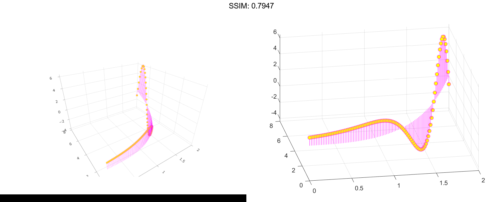
X = linspace(0,2); Y = X.^3; Z = exp(X).*cos(Y); h = stem3(X,Y,Z,'filled');
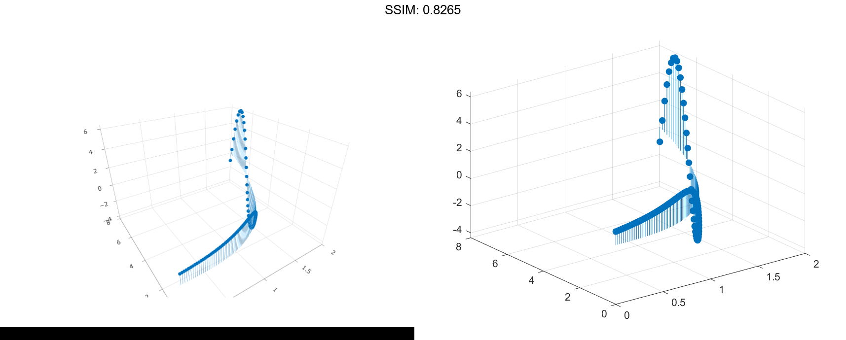
Change the color to magenta and set the marker face color to yellow. Use view to adjust the angle of the axes in the figure. Use dot notation to set properties.
h.Color = 'm';
h.MarkerFaceColor = 'y';
view(-10,35)

fig2plotly()
