geom_histogram

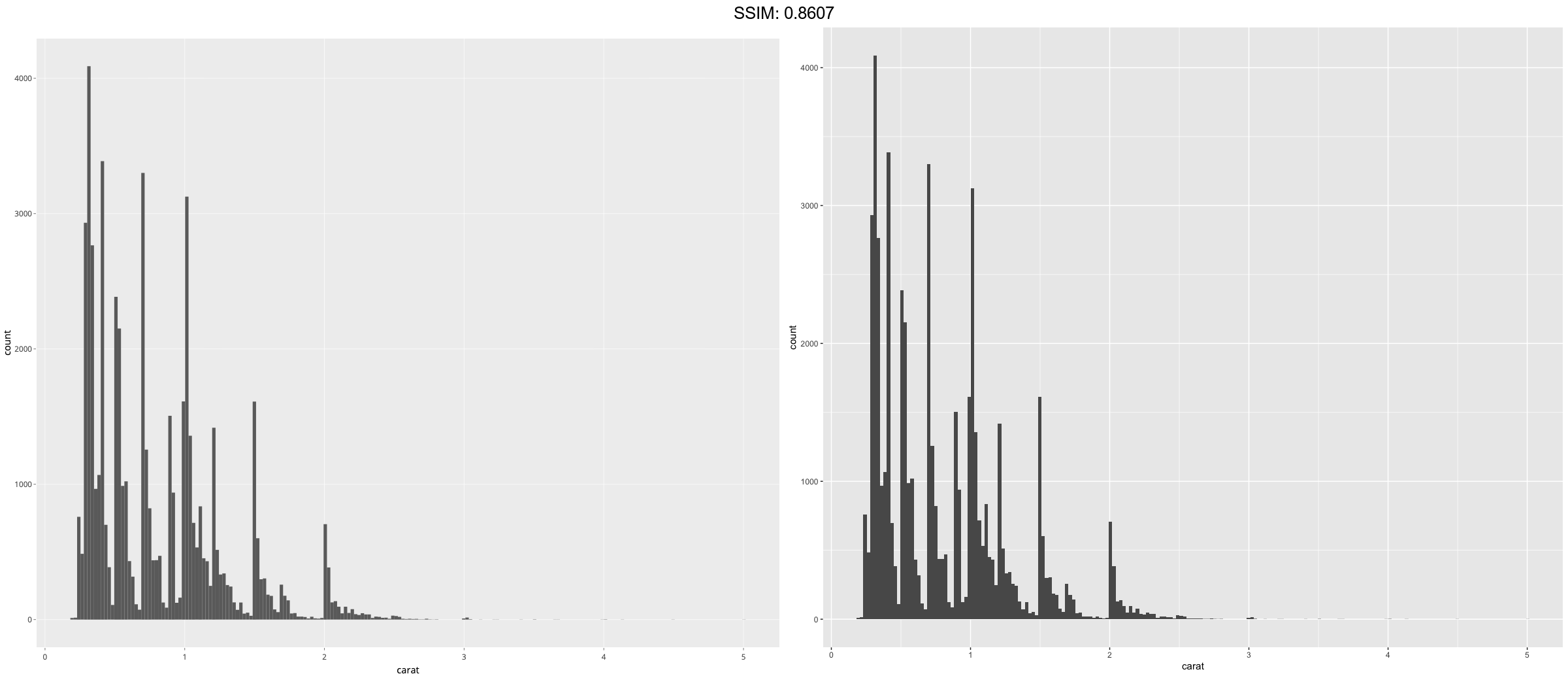
Visualise the distribution of a single continuous variable by dividing the x axis into bins and counting the number of observations in each bin and then convert them with ggplotly

p <-    
 ggplot(diamonds, aes(carat)) +
  geom_histogram()

plotly::ggplotly(p)

## `stat_bin()` using `bins = 30`. Pick better value with `binwidth`.

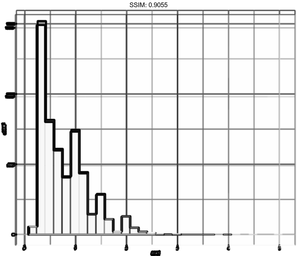
p <-    
 ggplot(diamonds, aes(carat)) +
  geom_histogram(binwidth = 0.01)

plotly::ggplotly(p)

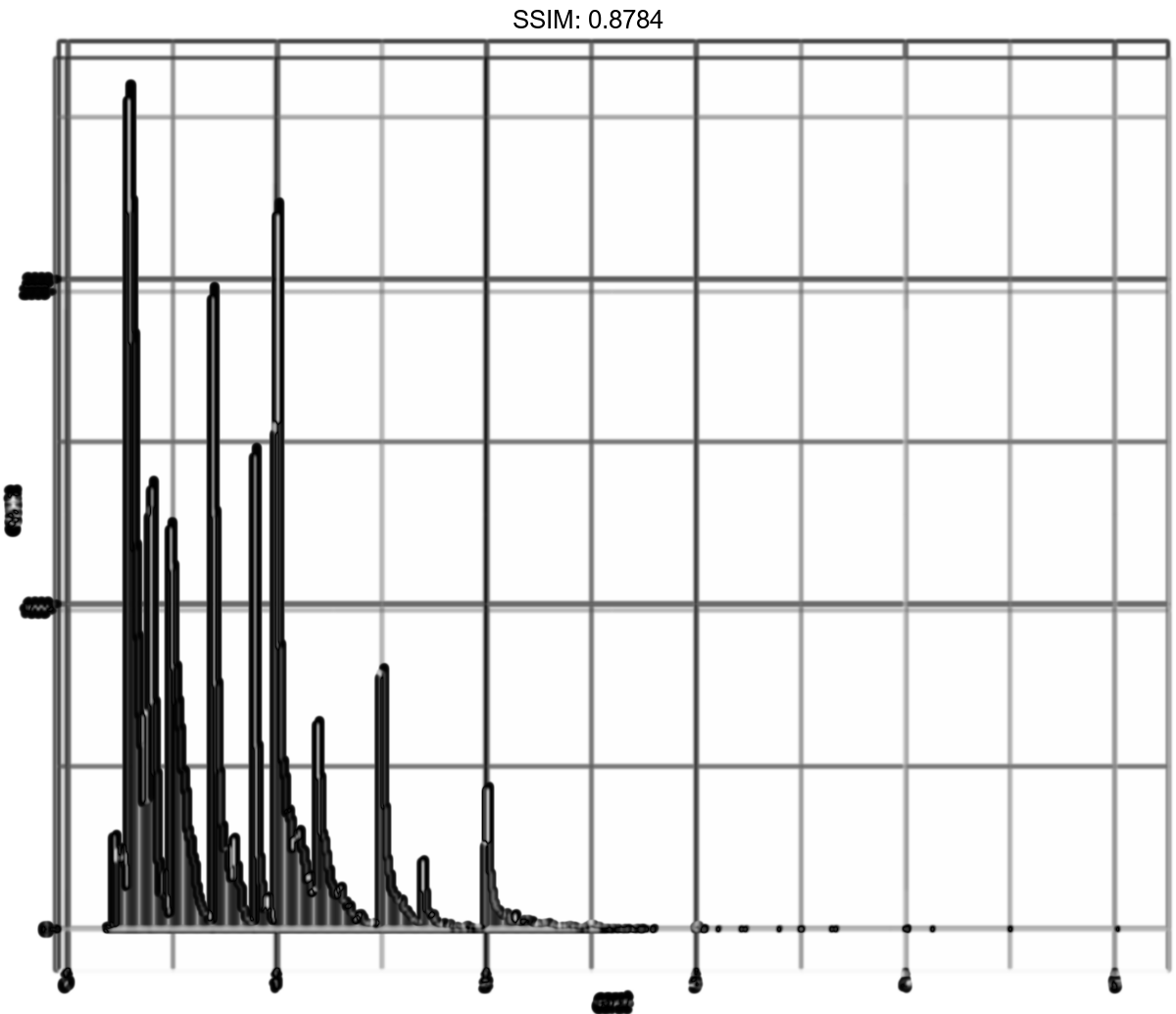
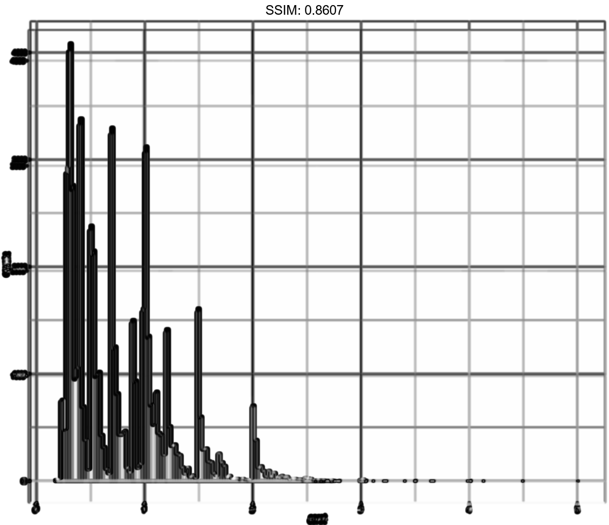
p <-    
 ggplot(diamonds, aes(carat)) +
  geom_histogram(bins = 200)

plotly::ggplotly(p)

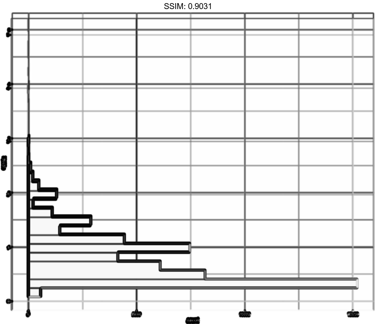
p <-    
 ggplot(diamonds, aes(y = carat)) +
  geom_histogram()

plotly::ggplotly(p)

## `stat_bin()` using `bins = 30`. Pick better value with `binwidth`.

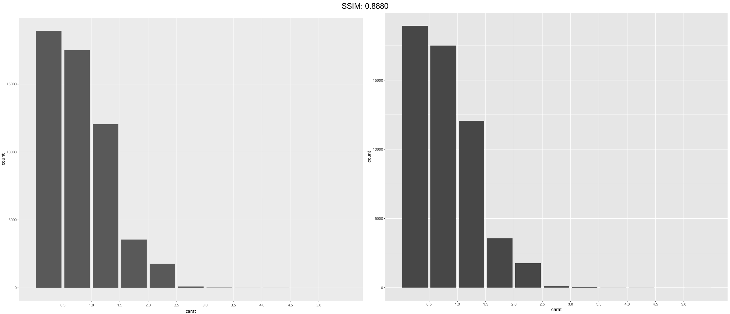
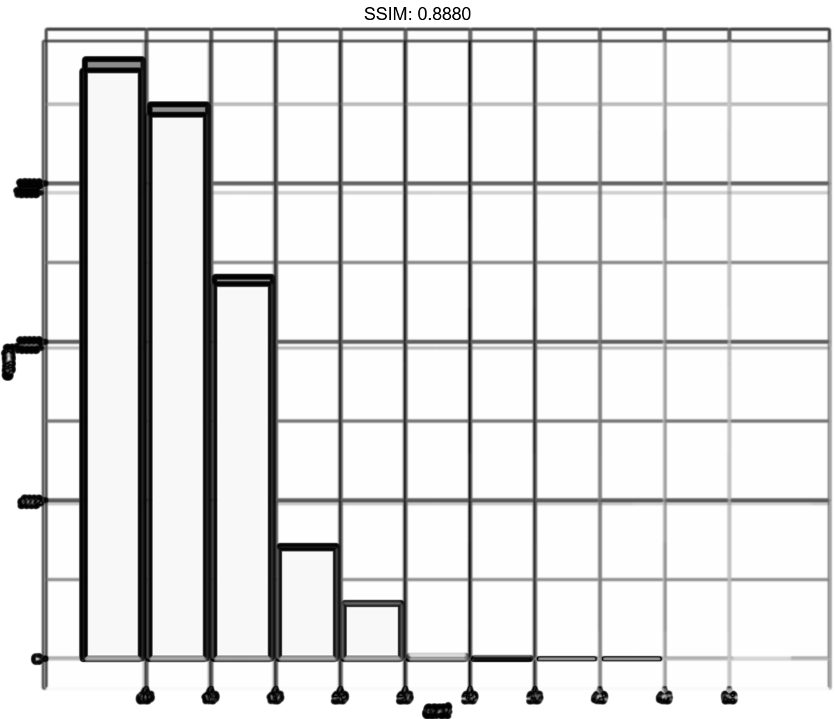
p <-    
 ggplot(diamonds, aes(carat)) +
  geom_bar() +
  scale_x_binned()

plotly::ggplotly(p)

p <-    
 ggplot(diamonds, aes(price, fill = cut)) +
  geom_histogram(binwidth = 500)

plotly::ggplotly(p)

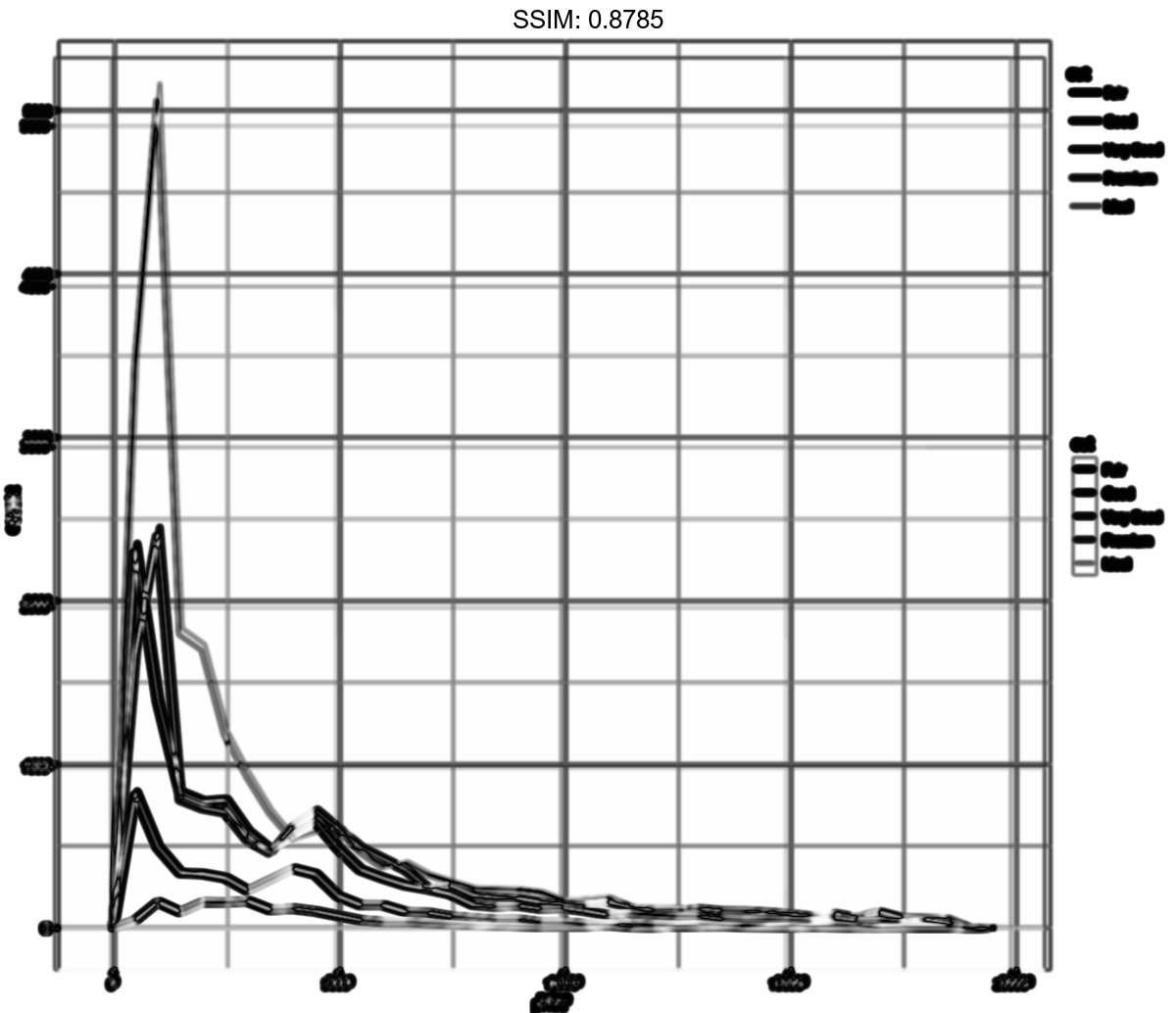
p <-    
 ggplot(diamonds, aes(price, colour = cut)) +
  geom_freqpoly(binwidth = 500)

plotly::ggplotly(p)

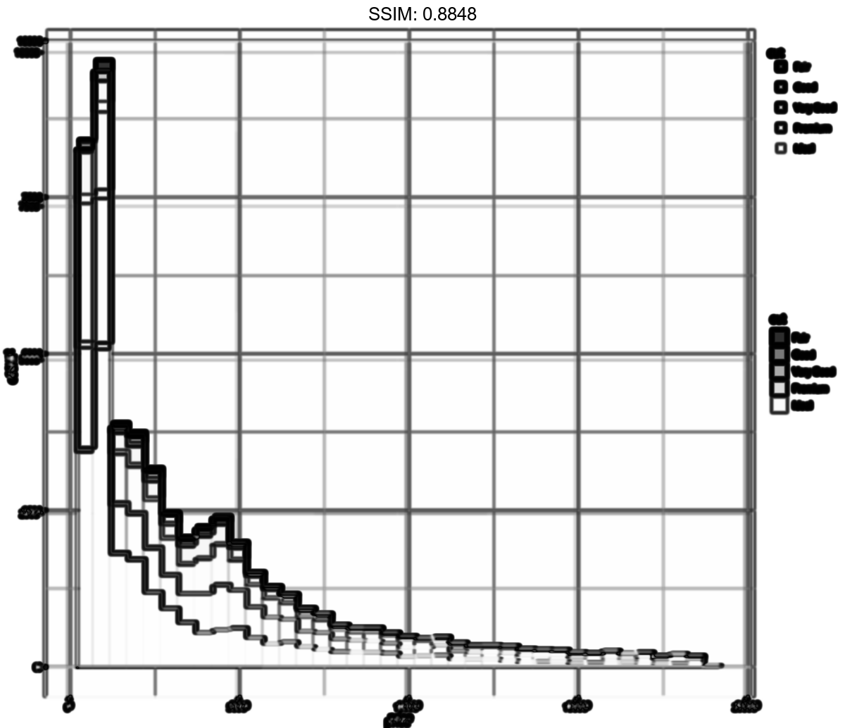
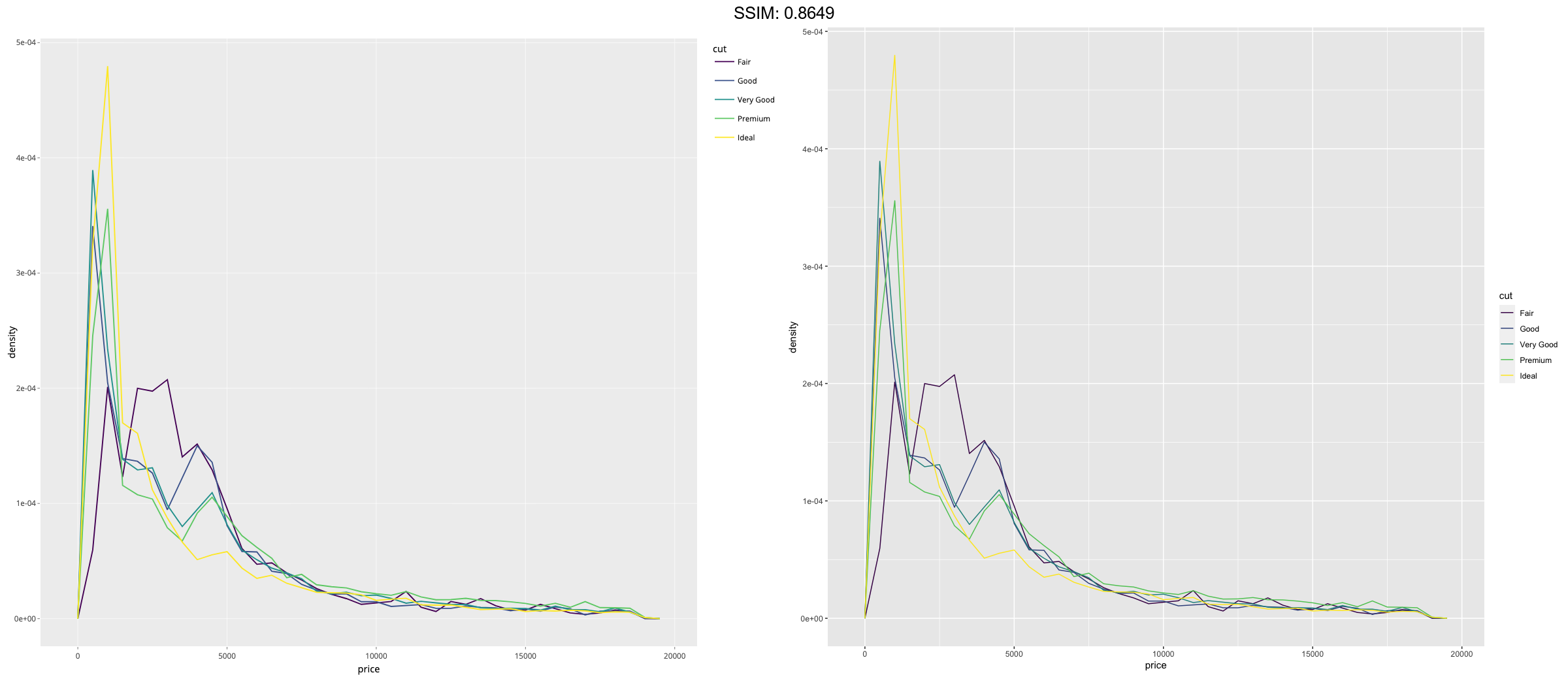
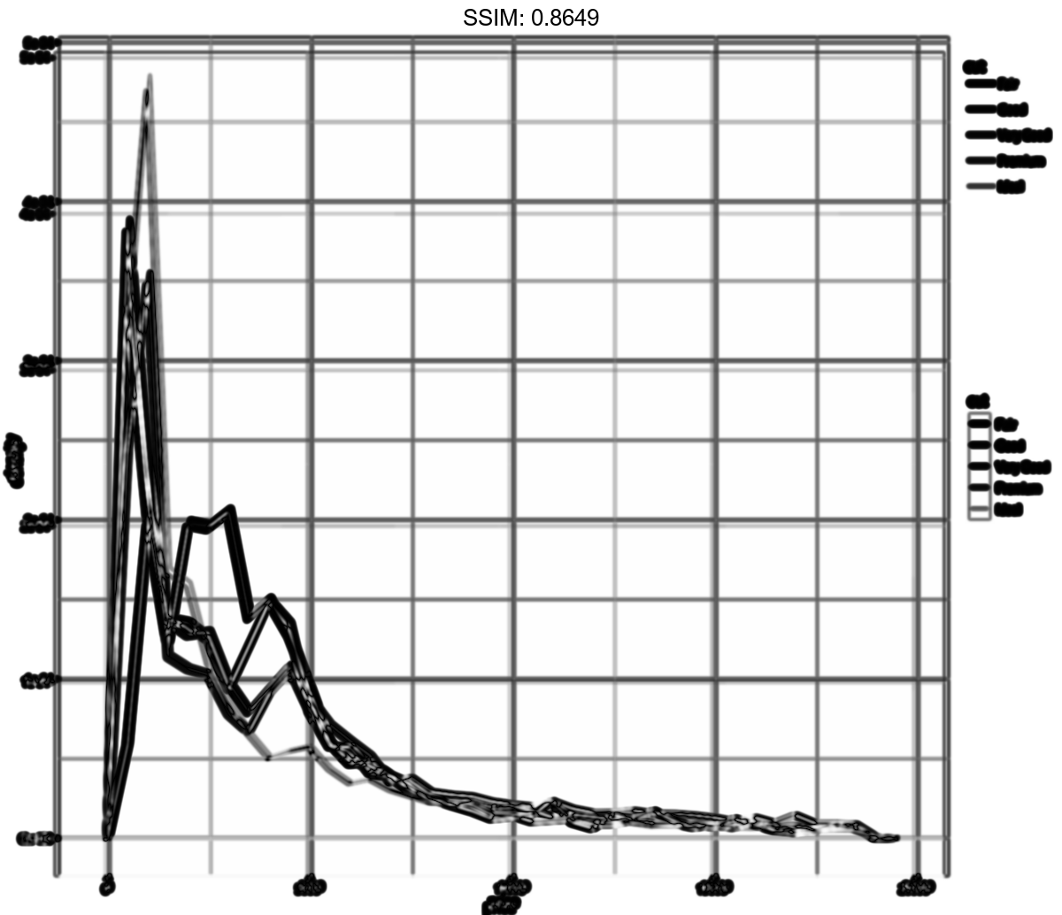
p <-    
 ggplot(diamonds, aes(price, after_stat(density), colour = cut)) +
  geom_freqpoly(binwidth = 500)

plotly::ggplotly(p)

p <-    
 if (require("ggplot2movies")) {
m <- ggplot(movies, aes(rating))
m + geom_histogram(binwidth = 0.1)
m +
  geom_histogram(aes(weight = votes), binwidth = 0.1) +
  ylab("votes")
m +
 geom_histogram() +
 scale_x_log10()
m +
  geom_histogram(binwidth = 0.05) +
  scale_x_log10()
m +
  geom_histogram(boundary = 0) +
  coord_trans(x = "log10")
m +
  geom_histogram(boundary = 0) +
  coord_trans(x = "sqrt")
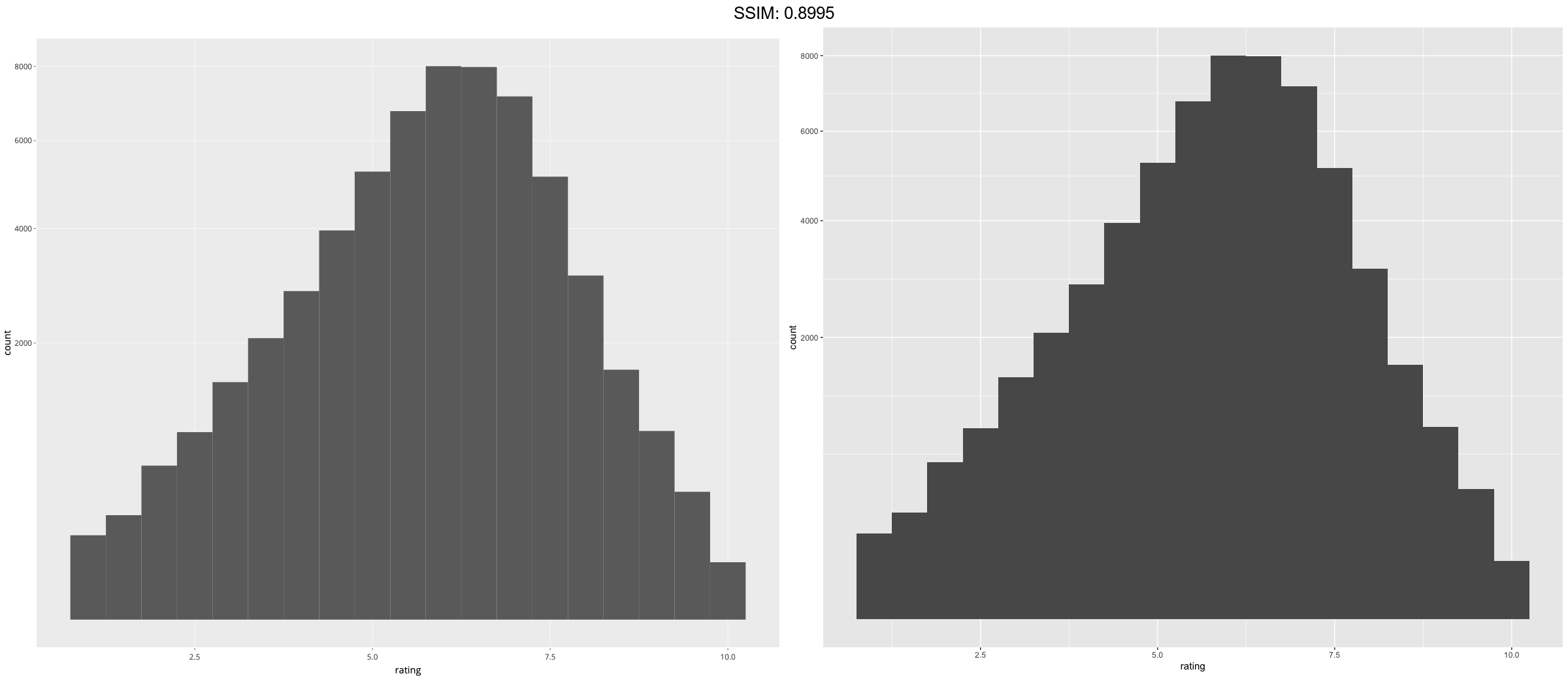
m <- ggplot(movies, aes(x = rating))
m +
  geom_histogram(binwidth = 0.5) +
  scale_y_sqrt()
}

plotly::ggplotly(p)

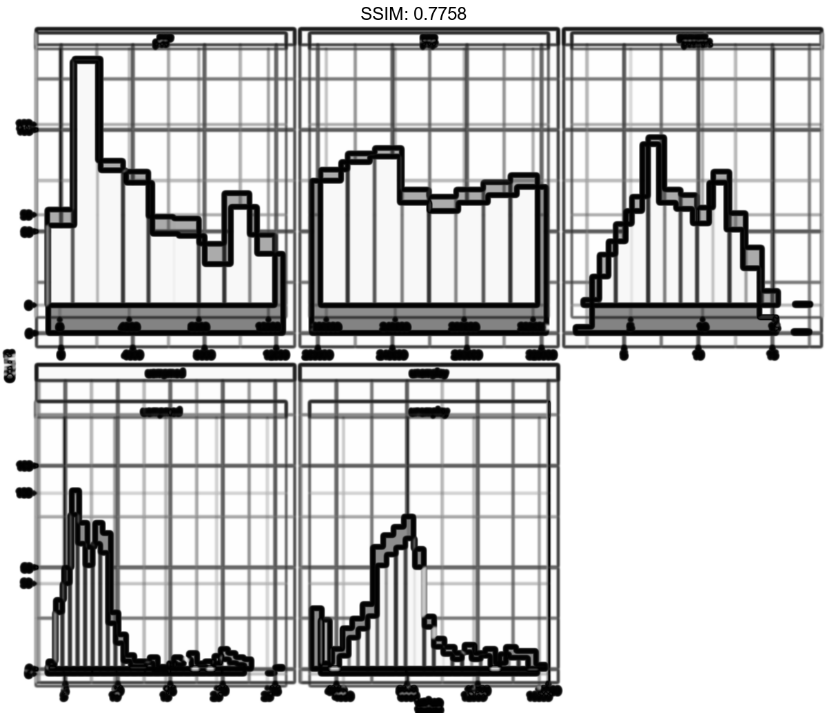
p <-    
 ggplot(economics_long, aes(value)) +
  facet_wrap(~variable, scales = 'free_x') +
  geom_histogram(binwidth = function(x) 2 * IQR(x) / (length(x)^(1/3)))

plotly::ggplotly(p)

GGPLOT - geom_histogram

GGPLOT - `geom_histogram`